24th January, 2018
What is a population?

- Individual genes, sequence fragments
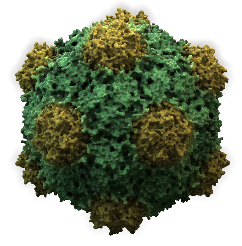
- Microscopic pathogens
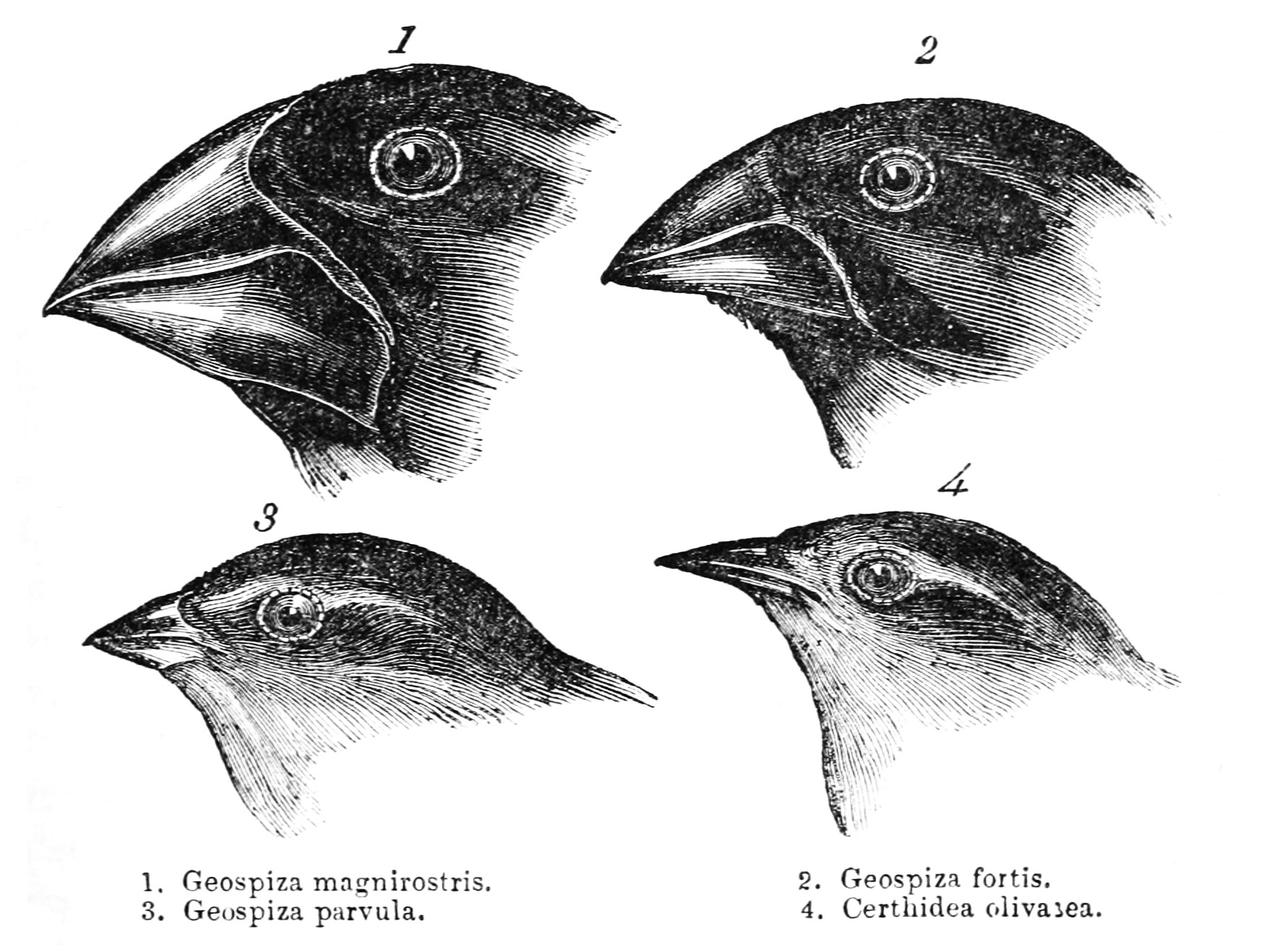
- Macroscopic biological organisms
- Groups of organisms
- Entire species

Demographic inference
Why involve genetics?


Genetic samples yield trees: information about events ancestral to samples.Ancestral event times may be informative when sample times aren't.
Bayesian Inference
What is probability?
We use the following definition of probability:For propositions $A$ and $B$, the probabiltiy $P(A|B)$ is the degree to which $A$ is believed to be true, on the condition that $B$ is true.
- Who is doing the believing?
- Probability is subjective.

Manipulating probabilities
There are only two rules for manipulating probabilities:
- The product rule: $$P(A|B,C)P(B|C) = P(A,B|C)$$ where $A,B$ represents $A$ and $B$.
- The sum rule: $$P(A|B) + P(\bar{A}|B) = 1$$ where $\bar{A}$ represents not $A$.
That's it! You can now do Bayesian statistics.
Bayes' rule
Suppose we have a probabilistic model $M$ with parameters $\theta_M$. Given data $D$ which we assume has been generated by the model, what can we learn about the parameters?
- Our model allows us to evaluate $P(D|M,\theta_M)$.
- We want to know $P(\theta_M|D,M)$.
Mechanically applying the product rule yields
$$\color{darkred}{P(\theta_M|D,M)} = \frac{\color{yellow}{P(D|M,\theta_M)}\color{darkblue}{P(\theta_M|M)}}{P(D|M)}$$
Terms are named posterior, likelihood and prior.
Bayesian inference
Bayes' rule gives us a natural framework for drawing on many sources of information:
- $\color{darkblue}{P(\theta_M|M)}$ describes our state of knowledge of $\theta_M$ prior to receiving $D$. (May still depend on expert knowledge.)
- $\color{#a0a000}{P(D|\theta,M_{\theta})}$ is the likelihood of $\theta_M$ given $D$. Describes how the data modifies our knowledge of $\theta_M$.
- $\color{red}{P(\theta_M|D,M)}$ describes our state of knowledge after receiving $D$.
The posterior of one analysis may be the prior of a second.
Bayesian credible intervals
For probability distributions/densities of a single variable, it is often useful to summarize the uncertainty in the value using an interval. This is the 95% highest posteriod density (HPD) interval:

Interpretation is easy: 95% posterior probability that the truth lies within this interval.
Bayesian phylogenetic inference
The Phylogenetic Likelihood
$$\LARGE P(A|T,\mu)$$
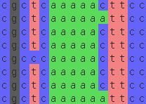
- $A$ is a multiple sequence alignment of $n$ sequences,
- $T$ is a phylogenetic tree with $n$ leaves, and
- $\mu$ are the parameters of the chosen substitution model.
- Sites assumed to evolve independently, so likelihood is just a product of site pattern probabilities: note the obvious generalizations to multiple alignments that share a tree, or to phylogenetic networks that allow different sites to evolve under distinct trees.
We're Bayesians: we need a probability distribution for $T$!
The Phylogenetic Posterior
$$P(T,\mu,\theta|A) = \frac{1}{P(A)} P(A|T,\mu)P(T|\theta)P(\mu,\theta)$$
- $P(T|\theta)$ is the "tree prior" or "phylodynamic likelihood" parameterized by $\theta$.
- $P(\mu,\theta)=P(\mu)P(\theta)$ are the parameter priors.
Questions
- What is $P(A)$?
- Is the tree prior really a prior?
(I.e. does it depend on the data?)
The Neutrality Assumption
Because of the way we've factorized the joint probability for the data and model parameters, we are implicitly assuming that our alignment could have been produced in the following fashion:


Separating the process of tree generation from that of sequence evolution implies neutrality.
Tree Priors (Phylodynamic Liklihoods)
- Tree priors allow us to specify a generative model for the genealogy.
- While this model may not involve genetic evolution, it may depend on speciation rates, population sizes, migration rates, etc. etc.
- A huge fraction of phylogenetics inference research is focused on developing and efficiently implementing tree priors!

Bayesian inference in practice
What's so difficult about this?
INTEGRATION
Bayes' theorem has a troublesome denominator: $$ P(\theta_M|D,M)=\frac{P(D|\theta_M,M)P(\theta_M|M)}{P(D|M)} $$
The quantity $P(D|M)$ is a normalizing constant, which is the result of integrating the numerator over all $\theta_M$: $$P(D|M)=\int P(D|\theta_M,M)P(\theta_M|M)d\theta_M$$
- Unless you're very lucky, you can't do this integral with pen and paper.
- If $\theta_M$ has many dimensions, you can't even do this using a computer.
Monte Carlo methods

Monte Carlo methods

Monte Carlo methods
In our context, Monte Carlo methods are algorithms which produce random samples of values in order to characterize a probability distribution over those values.
Usually, the algorithms we deal with seek to produce an arbitrary number of independent samples of $\theta_M$ drawn from the posterior distribution $P(\theta_M|D,M)$.
The Metropolis-Hastings algorithm
This algorithm produces samples from a distribution $f(x)$ by generating a random walk over possible values of $x$.


- walk explores mostly high probability areas
- algorithm does not require normalized $f(x)$
Metropolis-Hastings for trees
For phylogenetic inference, need to produce a random walk in the space of rooted time trees. A variety of different moves/"operators" are commonly used:

Result of MCMC algorithm


Convergence and Mixing
- Adjacent MCMC samples for $x$ are correlated.
- In the limit of an infinite number of steps between a pair of samples, they will be independent draws.
- The first state of the MCMC chain is chosen arbitrarily - it is not a draw from the posterior.

What determines convergence and mixing rates?
- Convergence is affected by the starting state.
- Convergence and mixing are affected by
- Proposals: how big are the steps in the random walk? What direction are they in?
- The target density: multiple modes cause havoc!
Assessing Convergence
The tried and true method for assessing convergence is to compare the results of distinct chains generated from independently selected initial conditions.
- Once satisfied, chains can be combined.
- Can run at the same time on a cluster.
- Doesn't necessarily prove convergence!
Assessing Mixing
The key to assessing mixing is the autocorrelation function of the chain states: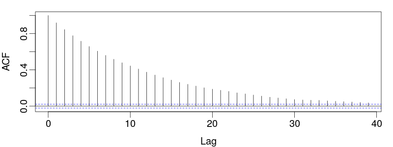
The number of steps required for this function to decay to within the vicinity of 0 is the gap between effectively independent samples, $\tau$.
Assessing Mixing (continued)
If $N$ is the total number of MCMC samples, we then define $$N_{\text{eff}}=\frac{N}{\tau}$$ to be the effective sample size (ESS).The ESS is a rough estimate of the number of actual samples a chain has generated.
You should really only consider the order of magnitude of the ESS.
Phylogenetic MCMC stopping criteria
- How can we tell when a phylogenetic MCMC calculation has reached equilibrium?
- How do we know when we've collected enough samples?
- One approach is to compute ESS estimates for each parameter
and a number of tree summary statistics (e.g. tree height and
tree "length" — sum of all edge lengths).
- Assume that once all of these scores are sufficiently high (e.g. > 200) we have adequately sampled the posterior.
- Examine output of several independent (and independently
initialized chains. A necessary (not sufficient) condition for
convergence is that sample distributions converge as the chains
converge to equilibrium.
- Always do this!
Demographic inference
Wright-Fisher model

- Discrete generations, fixed population size.
- Children from a given generation each select a parent uniformly at random from generation $\implies$ panmixia.
- Average birth-rate per individual is 1 child per generation.
- Average number of pairs per individual per generation is 0.5 pairs per generation.
Kingman's Coalescent

- Consider $k$ lineages which are ancestral to sampled individuals.
- There are $\binom{k}{2}$ potential pairings between sampled lineageages, compared to $\binom{N}{2}$ possible pairings between all individuals in the population.
- Every pair produced by a WF parent has probability $p_c(k)=\binom{k}{2}/\binom{N}{2}$ of involving a pair of our ancestral lineages.
- In limit $N\gg k$, coalescence probability per generation is $N\times0.5\times p_c=\binom{k}{2}\frac{1}{N}$.
- Coalescence rate per unit time is then $\binom{k}{2}\frac{1}{Ng}$ where $g$ is the generation time.
Kingman's Coalescent

- Backward-time Markov process that generates rooted time trees.
- Probability of tree under model is $$P(T|Ng)=\exp\left[-\Delta t_1\binom{k_1}{2}\frac{1}{Ng}\right]\frac{1}{Ng}\times\exp\left[-\Delta t_2\binom{k_2}{2}\frac{1}{Ng}\right]\frac{1}{Ng}\times\ldots$$
- I.e. waiting times drawn from exponential distributions of mean $Ng/\binom{k}{2}$.
Parametric population size inference
- It is possible to generalize the Wright-Fisher model to the case where population size is time dependent, i.e. $N(t)$. (Griffiths & Tavaré, 1994.)
- The corresponding coalescent distribution replaces the exponentially distributed waiting times with: $$P(t_{i+1}-t_i=\Delta t|k_i)=\exp\left[-\binom{k_i}{2}\int_{t_i}^{t_{i+1}}\frac{dt}{N(t)g}\right]\binom{k_i}{2}\frac{1}{Ng}$$
- Such phylodynamic models are useful for selecting between qualitatively distinct hypotheses.
- More recently, this approach has been extended by to account for population dynamics which arise as the result of birth-death processes in the coalescent limit. (Volz et al., 2009)
- This is suitable for parametric inference when the underlying population dynamics are understood (and the coalescent limit is appropriate).
But what if we know nothing about the dynamics?
Non-parametric inference

- Introduced by Pybus, Rambaut and Harvey (2000).
- Piecewise constant coalescent estimates may be interpreted as estimates of the harmonic mean of the population size within each interval.
- Maximum-likelihood estimates from fixed tree yield a remarkably robust and cheap means of demographic inference.
The Bayesian Skyline Plot


- Due to Drummond et al., 2005, applies generalized skyline plot (Strimmer and Pybus, 2001) as a tree prior for Bayesian inference of population dynamics.
- Requires specifying a group size parameter.
The Extended Bayesian Skyline Plot

- Method of Heled and Drummond (2008) which avoids specifying a group size and allows inference from multiple loci.
- Each coalescent is a potential population gradient switch event, a decision which is inferred separately for each event.
The Extended Bayesian Skyline Plot

- Distributing roughly the same number of samples across multiple loci yields dramatically improves the potential depth of the history that can be probed.
- (Antient DNA or serial sampling yields additional benefits.)
BEAST 2
BEAST 2 is a free (as in freedom) software package that uses MCMC to perform Bayesian phylogenetic inference.
Project website: beast2.org
- Download software
- Documentation and FAQs
- Tutorials
- ...
Fork/rewrite of BEAST 1.x, which is now a separately-maintained project. (Important to specify BEAST 1 or 2 when asking for help!)
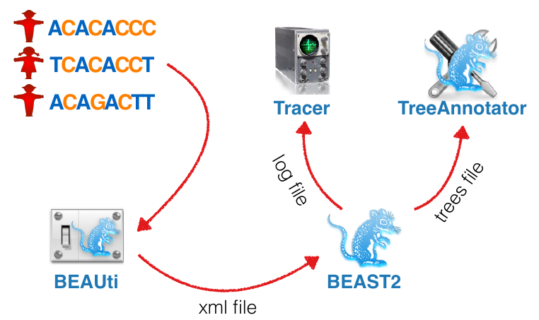
BEAST components (and friends)
- BEAST2: Software implementing MCMC for model parameter and tree inference
- BEAUti: GUI for setting up the input file
- Tracer: Tool for summarizing parameter posteriors
- Tree Annotator: Tool for summarizing tree posteriors
- FigTree: Tool for visualising trees
- ...
BEAST Workflow
Tutorial: EBSP
- Download tutorial material for the EBSP tutorial from the BEAST 2 Český Krumlov page at beast2.org/ceskykrumlov2018.
- Extract the ZIP file.
- Open the PDF file "ebsp2-tut.pdf" and follow the instructions.
- I will wrap up the tutorial 10-15 minutes before the end of the session.
Begin!