1Lagrangian Mechanics
The purpose of mechanics is to describe how bodies change their position in space with “time.” I should load my conscience with grave sins against the sacred spirit of lucidity were I to formulate the aims of mechanics in this way, without serious reflection and detailed explanations. Let us proceed to disclose these sins.
Albert Einstein, Relativity, the Special and General Theory [16], p. 9
The subject of this book is motion and the mathematical tools used to describe it.
Centuries of careful observations of the motions of the planets revealed regularities in those motions, allowing accurate predictions of phenomena such as eclipses and conjunctions. The effort to formulate these regularities and ultimately to understand them led to the development of mathematics and to the discovery that mathematics could be effectively used to describe aspects of the physical world. That mathematics can be used to describe natural phenomena is a remarkable fact.
A pin thrown by a juggler takes a rather predictable path and rotates in a rather predictable way. In fact, the skill of juggling depends crucially on this predictability. It is also a remarkable discovery that the same mathematical tools used to describe the motions of the planets can be used to describe the motion of the juggling pin.
Classical mechanics describes the motion of a system of particles, subject to forces describing their interactions. Complex physical objects, such as juggling pins, can be modeled as myriad particles with fixed spatial relationships maintained by stiff forces of interaction.
There are many conceivable ways a system could move that never occur. We can imagine that the juggling pin might pause in midair or go fourteen times around the head of the juggler before being caught, but these motions do not happen. How can we distinguish motions of a system that can actually occur from other conceivable motions? Perhaps we can invent some mathematical function that allows us to distinguish realizable motions from among all conceivable motions.
The motion of a system can be described by giving the position of every piece of the system at each moment. Such a description of the motion of the system is called a configuration path; the configuration path specifies the configuration as a function of time. The juggling pin rotates as it flies through the air; the configuration of the juggling pin is specified by giving the position and orientation of the pin. The motion of the juggling pin is specified by giving the position and orientation of the pin as a function of time.
The path-distinguishing function that we seek takes a configuration path as an input and produces some output. We want this function to have some characteristic behavior when its input is a realizable path. For example, the output could be a number, and we could try to arrange that this number be zero only on realizable paths. Newton's equations of motion are of this form; at each moment Newton's differential equations must be satisfied.
However, there is an alternate strategy that provides more insight and power: we could look for a path-distinguishing function that has a minimum on the realizable paths—on nearby unrealizable paths the value of the function is higher than it is on the realizable path. This is the variational strategy: for each physical system we invent a path-distinguishing function that distinguishes realizable motions of the system by having a stationary point for each realizable path.1 For a great variety of systems realizable motions of the system can be formulated in terms of a variational principle.2
Mechanics, as invented by Newton and others of his era, describes the motion of a system in terms of the positions, velocities, and accelerations of each of the particles in the system. In contrast to the Newtonian formulation of mechanics, the variational formulation of mechanics describes the motion of a system in terms of aggregate quantities that are associated with the motion of the system as a whole.
In the Newtonian formulation the forces can often be written as derivatives of the potential energy of the system. The motion of the system is determined by considering how the individual component particles respond to these forces. The Newtonian formulation of the equations of motion is intrinsically a particle-by-particle description.
In the variational formulation the equations of motion are formulated in terms of the difference of the kinetic energy and the potential energy. The potential energy is a number that is characteristic of the arrangement of the particles in the system; the kinetic energy is a number that is determined by the velocities of the particles in the system. Neither the potential energy nor the kinetic energy depends on how those positions and velocities are specified. The difference is characteristic of the system as a whole and does not depend on the details of how the system is specified. So we are free to choose ways of describing the system that are easy to work with; we are liberated from the particle-by-particle description inherent in the Newtonian formulation.
The variational formulation has numerous advantages over the Newtonian formulation. The equations of motion for those parameters that describe the state of the system are derived in the same way regardless of the choice of those parameters: the method of formulation does not depend on the choice of coordinate system. If there are positional constraints among the particles of a system the Newtonian formulation requires that we consider the forces maintaining these constraints, whereas in the variational formulation the constraints can be built into the coordinates. The variational formulation reveals the association of conservation laws with symmetries. The variational formulation provides a framework for placing any particular motion of a system in the context of all possible motions of the system. We pursue the variational formulation because of these advantages.
1.1 Configuration Spaces
Let us consider mechanical systems that can be thought of as composed of constituent point particles, with mass and position, but with no internal structure.3 Extended bodies may be thought of as composed of a large number of these constituent particles with specific spatial relationships among them. Extended bodies maintain their shape because of spatial constraints among the constituent particles. Specifying the position of all the constituent particles of a system specifies the configuration of the system. The existence of constraints among parts of the system, such as those that determine the shape of an extended body, means that the constituent particles cannot assume all possible positions. The set of all configurations of the system that can be assumed is called the configuration space of the system. The dimension of the configuration space is the smallest number of parameters that have to be given to completely specify a configuration. The dimension of the configuration space is also called the number of degrees of freedom of the system.4
For a single unconstrained particle it takes three parameters to specify the configuration; a point particle has a three-dimensional configuration space. If we are dealing with a system with more than one point particle, the configuration space is more complicated. If there are k separate particles we need 3k parameters to describe the possible configurations. If there are constraints among the parts of a system the configuration is restricted to a lower-dimensional space. For example, a system consisting of two point particles constrained to move in three dimensions so that the distance between the particles remains fixed has a five-dimensional configuration space: thus with three numbers we can fix the position of one particle, and with two others we can give the position of the other particle relative to the first.
Consider a juggling pin. The configuration of the pin is specified if we give the positions of the atoms making up the pin. However, there exist more economical descriptions of the configuration. In the idealization that the juggling pin is truly rigid, the distances among all the atoms of the pin remain constant. So we can specify the configuration of the pin by giving the position of a single atom and the orientation of the pin. Using the constraints, the positions of all the other constituents of the pin can be determined from this information. The dimension of the configuration space of the juggling pin is six: the minimum number of parameters that specify the position in space is three, and the minimum number of parameters that specify an orientation is also three.
As a system evolves with time, the constituent particles move subject to the constraints. The motion of each constituent particle is specified by describing the changing configuration. Thus, the motion of the system may be described as evolving along a path in configuration space. The configuration path may be specified by a function, the configuration-path function, which gives the configuration of the system at any time.
Exercise 1.1: Degrees of freedom
For each of the mechanical systems described below, give the number of degrees of freedom of the configuration space.
a. Three juggling pins.
b. A spherical pendulum, consisting of a point mass (the pendulum bob) hanging from a rigid massless rod attached to a fixed support point. The pendulum bob may move in any direction subject to the constraint imposed by the rigid rod. The point mass is subject to the uniform force of gravity.
c. A spherical double pendulum, consisting of one point mass hanging from a rigid massless rod attached to a second point mass hanging from a second massless rod attached to a fixed support point. The point masses are subject to the uniform force of gravity.
d. A point mass sliding without friction on a rigid curved wire.
e. A top consisting of a rigid axisymmetric body with one point on the symmetry axis of the body attached to a fixed support, subject to a uniform gravitational force.
f. The same as e, but not axisymmetric.
1.2 Generalized Coordinates
In order to be able to talk about specific configurations we need to have a set of parameters that label the configurations. The parameters used to specify the configuration of the system are called the generalized coordinates. Consider an unconstrained free particle. The configuration of the particle is specified by giving its position. This requires three parameters. The unconstrained particle has three degrees of freedom. One way to specify the position of a particle is to specify its rectangular coordinates relative to some chosen coordinate axes. The rectangular components of the position are generalized coordinates for an unconstrained particle. Or consider an ideal planar double pendulum: a point mass constrained to be a given distance from a fixed point by a rigid rod, with a second mass constrained to be at a given distance from the first mass by another rigid rod, all confined to a vertical plane. The configuration is specified if the orientation of the two rods is given. This requires at least two parameters; the planar double pendulum has two degrees of freedom. One way to specify the orientation of each rod is to specify the angle it makes with a vertical plumb line. These two angles are generalized coordinates for the planar double pendulum.
The number of coordinates need not be the same as the dimension of the configuration space, though there must be at least that many. We may choose to work with more parameters than necessary, but then the parameters will be subject to constraints that restrict the system to possible configurations, that is, to elements of the configuration space.
For the planar double pendulum described above, the two angle coordinates are enough to specify the configuration. We could also take as generalized coordinates the rectangular coordinates of each of the masses in the plane, relative to some chosen coordinate axes. These are also fine coordinates, but we would have to explicitly keep in mind the constraints that limit the possible configurations to the actual geometry of the system. Sets of coordinates with the same dimension as the configuration space are easier to work with because we do not have to deal with explicit constraints among the coordinates. So for the time being we will consider only formulations where the number of configuration coordinates is equal to the number of degrees of freedom; later we will learn how to handle systems with redundant coordinates and explicit constraints.
In general, the configurations form a space M of some dimension n. The n-dimensional configuration space can be parameterized by choosing a coordinate function χ that maps elements of the configuration space to n-tuples of real numbers.5 If there is more than one dimension, the function χ is a tuple of n independent coordinate functions6 χi, i = 0, …, n − 1, where each χi is a real-valued function defined on some region of the configuration space.7 For a given configuration m in the configuration space M the values χi(m) of the coordinate functions are the generalized coordinates of the configuration. These generalized coordinates permit us to identify points of the n-dimensional configuration space with n-tuples of real numbers.8 For any given configuration space, there are a great variety of ways to choose generalized coordinates. Even for a single point moving without constraints, we can choose rectangular coordinates, polar coordinates, or any other coordinate system that strikes our fancy.
The motion of the system can be described by a configuration path γ mapping time to configuration-space points. Corresponding to the configuration path is a coordinate path q = χ ∘ γ mapping time to tuples of generalized coordinates.9 If there is more than one degree of freedom the coordinate path is a structured object: q is a tuple of component coordinate path functions qi = χi ∘ γ. At each instant of time t, the values q(t) = (q0(t), …, qn−1(t)) are the generalized coordinates of a configuration.
The derivative Dq of the coordinate path q is a function10 that gives the rate of change of the configuration coordinates at a given time: Dq(t) = (Dq0(t), …, Dqn−1(t)). The rate of change of a generalized coordinate is called a generalized velocity.
Exercise 1.2: Generalized coordinates
For each of the systems in exercise 1.1, specify a system of generalized coordinates that can be used to describe the behavior of the system.
1.3 The Principle of Stationary Action
Let us suppose that for each physical system there is a path-distinguishing function that is stationary on realizable paths. We will try to deduce some of its properties.
Experience of motion
Our ordinary experience suggests that physical motion can be described by configuration paths that are continuous and smooth.11 We do not see the juggling pin jump from one place to another. Nor do we see the juggling pin suddenly change the way it is moving.
Our ordinary experience suggests that the motion of physical systems does not depend upon the entire history of the system. If we enter the room after the juggling pin has been thrown into the air we cannot tell when it left the juggler's hand. The juggler could have thrown the pin from a variety of places at a variety of times with the same apparent result as we walk through the door.12 So the motion of the pin does not depend on the details of the history.
Our ordinary experience suggests that the motion of physical systems is deterministic. In fact, a small number of parameters summarize the important aspects of the history of the system and determine its future evolution. For example, at any moment the position, velocity, orientation, and rate of change of the orientation of the juggling pin are enough to completely determine the future motion of the pin.
Realizable paths
From our experience of motion we develop certain expectations about realizable configuration paths. If a path is realizable, then any segment of the path is a realizable path segment. Conversely, a path is realizable if every segment of the path is a realizable path segment. The realizability of a path segment depends on all points of the path in the segment. The realizability of a path segment depends on every point of the path segment in the same way; no part of the path is special. The realizability of a path segment depends only on points of the path within the segment; the realizability of a path segment is a local property.
So the path-distinguishing function aggregates some local property of the system measured at each moment along the path segment. Each moment along the path must be treated in the same way. The contributions from each moment along the path segment must be combined in a way that maintains the independence of the contributions from disjoint subsegments. One method of combination that satisfies these requirements is to add up the contributions, making the path-distinguishing function an integral over the path segment of some local property of the path.13
So we will try to arrange that the path-distinguishing function, constructed as an integral of a local property along the path, assumes a stationary value for any realizable path. Such a path-distinguishing function is traditionally called an action for the system. We use the word “action” to be consistent with common usage. Perhaps it would be clearer to continue to call it “path-distinguishing function,” but then it would be more difficult for others to know what we were talking about.14
In order to pursue the agenda of variational mechanics, we must invent action functions that are stationary on the realizable trajectories of the systems we are studying. We will consider actions that are integrals of some local property of the configuration path at each moment. Let q = χ ∘ γ be a coordinate path in the configuration space; q(t) are the coordinates of the configuration at time t. Then the action of a segment of the path in the time interval from t1 to t2 is15
where F[q] is a function of time that measures some local property of the path. It may depend upon the value of the function q at that time and the value of any derivatives of q at that time.16
The configuration path can be locally described at a moment in terms of the coordinates, the rate of change of the coordinates, and all the higher derivatives of the coordinates at the given moment. Given this information the path can be reconstructed in some interval containing that moment.17 Local properties of paths can depend on no more than the local description of the path.
The function F measures some local property of the coordinate path q. We can decompose F [q] into two parts: a part that measures some property of a local description and a part that extracts a local description of the path from the path function. The function that measures the local property of the system depends on the particular physical system; the method of construction of a local description of a path from a path is the same for any system. We can write F[q] as a composition of these two functions:18
The function Γ takes the coordinate path and produces a function of time whose value is an ordered tuple containing the time, the coordinates at that time, the rate of change of the coordinates at that time, and the values of higher derivatives of the coordinates evaluated at that time. For the path q and time t:
We refer to this tuple, which includes as many derivatives as are needed, as the local tuple. The function Γ[q] depends only on the coordinate path q and its derivatives; the function Γ[q] does not depend on χ or the fact that q is made by composing χ with γ.
The function L depends on the specific details of the physical system being investigated, but does not depend on any particular configuration path. The function L computes a real-valued local property of the path. We will find that L needs only a finite number of components of the local tuple to compute this property: The path can be locally reconstructed from the full local description; that L depends on a finite number of components of the local tuple guarantees that it measures a local property.19
The advantage of this decomposition is that the local description of the path is computed by a uniform process from the configuration path, independent of the system being considered. All of the system-specific information is captured in the function L.
The function L is called a Lagrangian20 for the system, and the resulting action,
is called the Lagrangian action. For Lagrangians that depend only on time, positions, and velocities the action can also be written
Lagrangians can be found for a great variety of systems. We will see that for many systems the Lagrangian can be taken to be the difference between kinetic and potential energy. Such Lagrangians depend only on the time, the configuration, and the rate of change of the configuration. We will focus on this class of systems, but will also consider more general systems from time to time.
A realizable path of the system is to be distinguished from others by having stationary action with respect to some set of nearby unrealizable paths. Now some paths near realizable paths will also be realizable: for any motion of the juggling pin there is another that is slightly different. So when addressing the question of whether the action is stationary with respect to variations of the path we must somehow restrict the set of paths we are considering to contain only one realizable path. It will turn out that for Lagrangians that depend only on the configuration and rate of change of configuration it is enough to restrict the set of paths to those that have the same configuration at the endpoints of the path segment.
The principle of stationary action asserts that for each dynamical system we can cook up a Lagrangian such that a realizable path connecting the configurations at two times t1 and t2 is distinguished from all conceivable paths by the fact that the action S[q](t1, t2) is stationary with respect to variations of the path.21 For Lagrangians that depend only on the configuration and rate of change of configuration, the variations are restricted to those that preserve the configurations at t1 and t2.22
Exercise 1.3: Fermat optics
Fermat observed that the laws of reflection and refraction could be accounted for by the following facts: Light travels in a straight line in any particular medium with a velocity that depends upon the medium. The path taken by a ray from a source to a destination through any sequence of media is a path of least total time, compared to neighboring paths. Show that these facts imply the laws of reflection and refraction.23
1.4 Computing Actions
To illustrate the above ideas, and to introduce their formulation as computer programs, we consider the simplest mechanical system—a free particle moving in three dimensions. Euler and Lagrange discovered that for a free particle the time integral of the kinetic energy over the particle's actual path is smaller than the same integral along any alternative path between the same points: a free particle moves according to the principle of stationary action, provided we take the Lagrangian to be the kinetic energy. The kinetic energy for a particle of mass m and velocity
Following Euler and Lagrange, the Lagrangian for the free particle is24
where the formal parameter x names a tuple of components of the position with respect to a given rectangular coordinate system, and the formal parameter v names a tuple of velocity components.25
We can express this formula as a procedure:
(define ((L-free-particle mass) local)
  (let ((v (velocity local)))
    (* 1/2 mass (dot-product v v))))
The definition indicates that L-free-particle is a procedure that takes mass as an argument and returns a procedure that takes a local tuple local, extracts the generalized velocity with the procedure velocity, and uses the velocity to compute the value of the Lagrangian.26
Suppose we let q denote a coordinate path function that maps time to position components:27
We can make this definition28
(define q
  (up (literal-function 'x)
      (literal-function 'y)
      (literal-function 'z)))
where literal-function makes a procedure that represents a function of one argument that has no known properties other than the given symbolic name. The symbol q now names a procedure of one real argument (time) that produces a tuple of three components representing the coordinates at that time. For example, we can evaluate this procedure for a symbolic time t as follows:
(q 't)(up (x t) (y t) (z t))The derivative of the coordinate path Dq is the function that maps time to velocity components:
We can make and use the derivative of a function.29 For example, we can write:
((D q) 't)(up ((D x) t) ((D y) t) ((D z) t))The function Γ takes a coordinate path and returns a function of time that gives the local tuple (t, q(t), Dq(t), …). We implement this Γ with the procedure Gamma.30 Here is what Gamma does:
((Gamma q) 't)(up t
(up (x t) (y t) (z t))
(up ((D x) t) ((D y) t) ((D z) t)))So the composition L ∘ Γ is a function of time that returns the value of the Lagrangian for this point on the path:31
((compose (L-free-particle 'm) (Gamma q)) 't)(+ (* 1/2 m (expt ((D x) t) 2))
(* 1/2 m (expt ((D y) t) 2))
(* 1/2 m (expt ((D z) t) 2)))The procedure show-expression simplifies the expression and uses TEX to display the result in traditional infix form. We use this method of display to make the boxed expressions in this book. The procedure show-expression also produces the prefix form, but we usually do not show this.32
(show-expression
((compose (L-free-particle 'm) (Gamma q)) 't))According to equation (1.4) we can compute the Lagrangian action from time t1 to time t2 as:
(define (Lagrangian-action L q t1 t2)
  (definite-integral (compose L (Gamma q)) t1 t2))
Lagrangian-action takes as arguments a procedure L that computes the Lagrangian, a procedure q that computes a coordinate path, and starting and ending times t1 and t2. The definite-integral used here takes as arguments a function and two limits t1 and t2, and computes the definite integral of the function over the interval from t1 to t2.33 Notice that the definition of Lagrangian-action does not depend on any particular set of coordinates or even the dimension of the configuration space. The method of computing the action from the coordinate representation of a Lagrangian and a coordinate path does not depend on the coordinate system.
We can now compute the action for the free particle along a path. For example, consider a particle moving at uniform speed along a straight line t ↦ (4t + 7, 3t + 5, 2t + 1).34 We represent the path as a procedure
(define (test-path t)
  (up (+ (* 4 t) 7)
      (+ (* 3 t) 5)
      (+ (* 2 t) 1)))
For a particle of mass 3, we obtain the action between t = 0 and t = 10 as35
(Lagrangian-action (L-free-particle 3.0)
test-path 0.0 10.0)435Exercise 1.4: Lagrangian actions
For a free particle an appropriate Lagrangian is36
Suppose that x is the constant-velocity straight-line path of a free particle, such that xa = x(ta) and xb = x(tb). Show that the action on the solution path is
Paths of minimum action
We already know that the actual path of a free particle is uniform motion in a straight line. According to Euler and Lagrange, the action is smaller along a straight-line test path than along nearby paths. Let q be a straight-line test path with action S[q](t1, t2). Let q + ϵη be a nearby path, obtained from q by adding a path variation η scaled by the real parameter ϵ.37 The action on the varied path is S[q + ϵη](t1, t2). Euler and Lagrange found that S[q + ϵη](t1, t2) > S[q](t1, t2) for any η that is zero at the endpoints and for any small nonzero ϵ.
Let's check this numerically by varying the test path, adding some amount of a test function that is zero at the endpoints t = t1 and t = t2. To make a function η that is zero at the endpoints, given a sufficiently well-behaved function ν, we can use η(t) = (t − t1)(t − t2)ν(t). This can be implemented:
(define ((make-eta nu t1 t2) t)
  (* (- t t1) (- t t2) (nu t)))
We can use this to compute the action for a free particle over a path varied from the given path, as a function of ϵ:38
(define ((varied-free-particle-action mass q nu t1 t2) eps)
  (let ((eta (make-eta nu t1 t2)))
    (Lagrangian-action (L-free-particle mass)
                       (+ q (* eps eta))
                       t1
                       t2)))
The action for the varied path, with ν(t) = (sin t, cos t, t2) and ϵ = 0.001, is, as expected, larger than for the test path:
((varied-free-particle-action 3.0 test-path
                              (up sin cos square)
                              0.0 10.0)
0.001)436.29121428571153We can numerically compute the value of ϵ for which the action is minimized. We search between, say, −2 and 1:39
(minimize
  (varied-free-particle-action 3.0 test-path
                               (up sin cos square)
                               0.0 10.0)
-2.0 1.0)(-1.5987211554602254e-14 435.0000000000237 5)We find exactly what is expected—that the best value for ϵ is zero,40 and the minimum value of the action is the action along the straight path.
Finding trajectories that minimize the action
We have used the variational principle to determine if a given trajectory is realizable. We can also use the variational principle to find trajectories. Given a set of trajectories that are specified by a finite number of parameters, we can search the parameter space looking for the trajectory in the set that best approximates the real trajectory by finding one that minimizes the action. By choosing a good set of approximating functions we can get arbitrarily close to the real trajectory.41
One way to make a parametric path that has fixed endpoints is to use a polynomial that goes through the endpoints as well as a number of intermediate points. Variation of the positions of the intermediate points varies the path; the parameters of the varied path are the coordinates of the intermediate positions. The procedure make-path constructs such a path using a Lagrange interpolation polynomial. The procedure make-path is called with five arguments: (make-path t0 q0 t1 q1 qs), where q0 and q1 are the endpoints, t0 and t1 are the corresponding times, and qs is a list of intermediate points.42
Having specified a parametric path, we can construct a parametric action that is just the action computed along the parametric path:
(define ((parametric-path-action Lagrangian t0 q0 t1 q1) qs)
  (let ((path (make-path t0 q0 t1 q1 qs)))
    (Lagrangian-action Lagrangian path t0 t1)))
We can find approximate solution paths by finding parameters that minimize the action. We do this minimization with a canned multidimensional minimization procedure:43
(define (find-path Lagrangian t0 q0 t1 q1 n)
  (let ((initial-qs (linear-interpolants q0 q1 n)))
    (let ((minimizing-qs
            (multidimensional-minimize
              (parametric-path-action Lagrangian t0 q0 t1 q1)
              initial-qs)))
      (make-path t0 q0 t1 q1 minimizing-qs))))
The procedure multidimensional-minimize takes a procedure (in this case the value of the call to parametric-path-action) that computes the function to be minimized (in this case the action) and an initial guess for the parameters. Here we choose the initial guess to be equally spaced points on a straight line between the two endpoints, computed with linear-interpolants.
To illustrate the use of this strategy, we will find trajectories of the harmonic oscillator, with Lagrangian44
for mass m and spring constant k. This Lagrangian is implemented by45
(define ((L-harmonic m k) local)
  (let ((q (coordinate local))
        (v (velocity local)))
    (- (* 1/2 m (square v)) (* 1/2 k (square q)))))
We can find an approximate path taken by the harmonic oscillator for m = 1 and k = 1 between q(0) = 1 and q(π/2) = 0 as follows:46
(define q
  (find-path (L-harmonic 1.0 1.0) 0.0 1.0 :pi/2 0.0 3))
We know that the trajectories of this harmonic oscillator, for m = 1 and k = 1, are
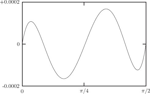
where the amplitude A and the phase φ are determined by the initial conditions. For the chosen endpoint conditions the solution is q(t) = cos(t). The approximate path should be an approximation to cosine over the range from 0 to π/2. Figure 1.1 shows the error in the polynomial approximation produced by this process. The maximum error in the approximation with three intermediate points is less than 1.7 × 10⁻⁴. We find, as expected, that the error in the approximation decreases as the number of intermediate points is increased. For four intermediate points it is about a factor of 15 better.
Exercise 1.5: Solution process
We can watch the progress of the minimization by modifying the procedure parametric-path-action to plot the path each time the action is computed. Try this:
(define win2 (frame 0.0 :pi/2 0.0 1.2))

(define ((parametric-path-action Lagrangian t0 q0 t1 q1)
         intermediate-qs)
  (let ((path (make-path t0 q0 t1 q1 intermediate-qs)))
    ;; display path
    (graphics-clear win2)
    (plot-function win2 path t0 t1 (/ (- t1 t0) 100))
    ;; compute action
    (Lagrangian-action Lagrangian path t0 t1)))

(find-path (L-harmonic 1.0 1.0) 0.0 1.0 :pi/2 0.0 2)
Exercise 1.6: Minimizing action
Suppose we try to obtain a path by minimizing an action for an impossible problem. For example, suppose we have a free particle and we impose endpoint conditions on the velocities as well as the positions that are inconsistent with the particle being free. Does the formalism protect itself from such an unpleasant attack? You may find it illuminating to program it and see what happens.
1.5 The Euler–Lagrange Equations
The principle of stationary action characterizes the realizable paths of systems in configuration space as those for which the action has a stationary value. In elementary calculus, we learn that the critical points of a function are the points where the derivative vanishes. In an analogous way, the paths along which the action is stationary are solutions of a system of differential equations. This system, called the Euler–Lagrange equations or just the Lagrange equations, is the link that permits us to use the principle of stationary action to compute the motions of mechanical systems, and to relate the variational and Newtonian formulations of mechanics.
Lagrange equations
We will find that if L is a Lagrangian for a system that depends on time, coordinates, and velocities, and if q is a coordinate path for which the action S[q](t1, t2) is stationary (with respect to any variation in the path that keeps the endpoints of the path fixed), then
Here L is a real-valued function of a local tuple; ∂1L and ∂2L denote the partial derivatives of L with respect to its generalized position argument and generalized velocity argument respectively.47 The function ∂2L maps a local tuple to a structure whose components are the derivatives of L with respect to each component of the generalized velocity. The function Γ[q] maps time to the local tuple: Γ[q](t) = (t, q(t), Dq(t), …). Thus the compositions ∂1L ∘ Γ[q] and ∂2L ∘ Γ[q] are functions of one argument, time. The Lagrange equations assert that the derivative of ∂2L ∘ Γ[q] is equal to ∂1L ∘ Γ[q], at any time. Given a Lagrangian, the Lagrange equations form a system of ordinary differential equations that must be satisfied by realizable paths.
Lagrange's equations are traditionally written as a separate equation for each component of q:
In this way of writing Lagrange's equations the notation does not distinguish between L, which is a real-valued function of three variables (t, q,
A correct use of the traditional notation is more explicit:
where i = 0, …, n − 1. In these equations we see that the partial derivatives of the Lagrangian function are taken, then the path and its derivative are substituted for the position and velocity arguments of the Lagrangian, resulting in an expression in terms of the time.
1.5.1 Derivation of the Lagrange Equations
We will show that the principle of stationary action implies that realizable paths satisfy the Euler–Lagrange equations.
A Direct Derivation
Let q be a realizable coordinate path from (t1, q(t1)) to (t2, q(t2)). Consider nearby paths q + ϵη where η(t1) = η(t2) = 0. Let
Expanding as a power series in ϵ
and using the chain rule we get
Integrating the second term by parts we obtain
The increment ΔS in the action due to the variation in the path is, to first order in ϵ, ϵDg(0). Because η is zero at the endpoints the integrated term is zero. Collecting together the other two terms, and reverting to functional notation, we find the increment to be
If ΔS is zero the action is stationary. We retain enough freedom in the choice of the variation that the factor in the integrand multiplying η is forced to be zero at each point along the path. We argue by contradiction: Suppose this factor were nonzero at some particular time. Then it would have to be nonzero in at least one of its components. But if we choose our η to be a bump that is nonzero only in that component in a neighborhood of that time, and zero everywhere else, then the integral will be nonzero. So we may conclude that the factor in curly brackets is identically zero and thus obtain Lagrange's equations:48
The Variation Operator
First we will develop tools for investigating how path-dependent functions vary as the paths are varied. We will then apply these tools to the action, to derive the Lagrange equations.
Suppose that we have a function f[q] that depends on a path q. How does the function vary as the path is varied? Let q be a coordinate path and q + ϵη be a varied path, where the function η is a path-like function that can be added to the path q, and the factor ϵ is a scale factor. We define the variation δηf[q] of the function f on the path q by49
The variation of f is a linear approximation to the change in the function f for small variations in the path. The variation of f depends on η.
A simple example is the variation of the identity path function: I[q] = q. Applying the definition, we find
It is traditional to write δηI[q] simply as δq. Another example is the variation of the path function that returns the derivative of the path. We have50
It is traditional to write δηg[q] as δDq.
The variation may be represented in terms of a derivative. Let g(ϵ) = f[q + ϵη]; then
Variations have the following derivative-like properties. For path-dependent functions f and g and constant c:
Let F be a path-independent function and g be a path-dependent function; then
The operators D (differentiation) and δ (variation) commute in the following sense:
Variations also commute with integration in a similar sense.
If a path-dependent function f is stationary for a particular path q with respect to small changes in that path, then it must be stationary for a subset of those variations that results from adding small multiples of a particular function η to q. So the statement δηf[q] = 0 for arbitrary η implies the function f is stationary for small variations of the path around q.
Exercise 1.7: Properties of δ
Show that δ has the properties 1.23–1.27.
Exercise 1.8: Implementation of δ
a. Suppose we have a procedure f that implements a path-dependent function: for path q and time t it has the value ((f q) t). The procedure delta computes the variation (δηf)[q](t) as the value of the expression ((((delta eta) f) q) t). Complete the definition of delta:
(define (((delta eta) f) q)
    ...
)
b. Use your delta procedure to verify the properties of δ listed in exercise 1.7 for simple functions such as implemented by the procedure f:51
(define (f q)
  (compose
    (literal-function 'F
                      (-> (UP Real (UP* Real) (UP* Real)) Real))
    (Gamma q)))
This implements an n-degree-of-freedom path-dependent function that depends on the local tuple of the path at each moment. You can define a literal two-dimensional path by
(define q (literal-function 'q (-> Real (UP Real Real))))
You should compute both sides of the equalities and subtract the results. The answer should be zero.
A Derivation with the Variation Operator
The action is the integral of the Lagrangian along a path:
For a realizable path q the variation of the action with respect to any variation η that preserves the endpoints, η(t1) = η(t2) = 0, is zero:
Variation commutes with integration, so the variation of the action is
Using the fact that
which follows from equations (1.20) and (1.21), and using the chain rule for variations (1.26), we get52
Integrating the last term of equation (1.32) by parts gives
For our variation η we have η(t1) = η(t2) = 0, so the first term vanishes.
Thus the variation of the action is zero if and only if
The variation of the action is zero because, by assumption, q is a realizable path. Thus (1.34) must be true for any function η that is zero at the endpoints. Since η is arbitrary, except for being zero at the endpoints, the bracketed factor of the integrand is zero. So
This is just what we set out to obtain, the Lagrange equations.
A path satisfying Lagrange's equations is one for which the action is stationary, and the fact that the action is stationary depends only on the values of L at each point of the path (and at each point on nearby paths), not on the coordinate system we use to compute these values. So if the system's path satisfies Lagrange's equations in some particular coordinate system, it must satisfy Lagrange's equations in any coordinate system. Thus the equations of variational mechanics are derived the same way in any configuration space and any coordinate system.
Harmonic oscillator
For an example, consider the harmonic oscillator. A Lagrangian is
Then
The Lagrangian is applied to a tuple of the time, a coordinate, and a velocity. The symbols t, x, and v are arbitrary; they are used to specify formal parameters of the Lagrangian.
Now suppose we have a configuration path y, which gives the coordinate of the oscillator y(t) for each time t. The initial segment of the corresponding local tuple at time t is
So
and
so the Lagrange equation is
which is the equation of motion of the harmonic oscillator.
Orbital motion
As another example, consider the two-dimensional motion of a particle of mass m orbiting a fixed center of attraction, with gravitational potential energy −μ/r, where r is the distance to the center of attraction. This is called the Kepler problem.
A Lagrangian for this problem is53
where ξ and η are formal parameters for rectangular coordinates of the particle, and vξ and vη are formal parameters for corresponding rectangular velocity components. Then
Similarly,
Now suppose we have a configuration path q = (x, y), so that the coordinate tuple at time t is q(t) = (x(t), y(t)). The initial segment of the local tuple at time t is
So
and
The component Lagrange equations at time t are
Exercise 1.9: Lagrange's equations
Derive the Lagrange equations for the following systems, showing all of the intermediate steps as in the harmonic oscillator and orbital motion examples.
a. An ideal planar pendulum consists of a bob of mass m connected to a pivot by a massless rod of length l subject to uniform gravitational acceleration g. A Lagrangian is
b. A particle of mass m moves in a two-dimensional potential V (x, y) = (x2 + y2)/2 + x2y − y3/3, where x and y are rectangular coordinates of the particle. A Lagrangian is
c. A Lagrangian for a particle of mass m constrained to move on a sphere of radius R is
Exercise 1.10: Higher-derivative Lagrangians
Derive Lagrange's equations for Lagrangians that depend on accelerations. In particular, show that the Lagrange equations for Lagrangians of the form L(t, q,
In general, these equations, first derived by Poisson, will involve the fourth derivative of q. Note that the derivation is completely analogous to the derivation of the Lagrange equations without accelerations; it is just longer. What restrictions must we place on the variations so that the critical path satisfies a differential equation?
1.5.2 Computing Lagrange's Equations
The procedure for computing Lagrange's equations mirrors the functional expression (1.12), where the procedure Gamma implements Γ:56
(define ((Lagrange-equations Lagrangian) q)
  (- (D (compose ((partial 2) Lagrangian) (Gamma q)))
     (compose ((partial 1) Lagrangian) (Gamma q))))
The argument of Lagrange-equations is a procedure that computes a Lagrangian. The Lagrange-equations procedure returns a procedure that when applied to a path q returns a procedure of one argument (time) that computes the left-hand side of the Lagrange equations (1.12). These residual values are zero if q is a path for which the Lagrangian action is stationary.
Observe that the Lagrange-equations procedure, like the Lagrange equations themselves, is valid for any generalized coordinate system. When we write programs to investigate particular systems, the procedures that implement the Lagrangian function and the path q will reflect the actual coordinates chosen to represent the system, but we use the same Lagrange-equations procedure in each case. This abstraction reflects the important fact that the method of derivation of Lagrange's equations from a Lagrangian is always the same; it is independent of the number of degrees of freedom, the topology of the configuration space, and the coordinate system used to describe points in the configuration space.
The free particle
Consider again the case of a free particle. The Lagrangian is implemented by the procedure L-free-particle. Rather than numerically integrating and minimizing the action, as we did in section 1.4, we can check Lagrange's equations for an arbitrary straight-line path t ↦ (at + a0, bt + b0, ct + c0):
(define (test-path t)
  (up (+ (* 'a t) 'a0)
      (+ (* 'b t) 'b0)
      (+ (* 'c t) 'c0)))

(((Lagrange-equations (L-free-particle 'm))
  test-path)
't)(down 0 0 0)That the residuals are zero indicates that the test path satisfies the Lagrange equations.57
We can also apply the Lagrange-equations procedure to an arbitrary function:58
(show-expression
  (((Lagrange-equations (L-free-particle 'm))
    (literal-function 'x))
   't))
(*(((expt D 2) x) t) m)The result is an expression containing the arbitrary time t and mass m, so it is zero precisely when D2x = 0, which is the expected equation for a free particle.
The harmonic oscillator
Consider the harmonic oscillator again, with Lagrangian (1.10). We know that the motion of a harmonic oscillator is a sinusoid with a given amplitude, frequency, and phase:
Suppose we have forgotten how the constants in the solution relate to the mass m and spring constant k of the oscillator. Let's plug in the proposed solution and look at the residual:
(define (proposed-solution t)
  (* 'A (cos (+ (* 'omega t) 'phi))))

(show-expression
  (((Lagrange-equations (L-harmonic 'm 'k))
    proposed-solution)
't))The residual here shows that for nonzero amplitude, the only solutions allowed are ones where (k − mω2) = 0 or
Exercise 1.11: Kepler's third law
A Lagrangian suitable for studying the relative motion of two particles, of masses m1 and m2, with potential energy V, is:
(define ((L-central-polar m V) local)
  (let ((q (coordinate local))
        (qdot (velocity local)))
    (let ((r (ref q 0))     (phi (ref q 1))
                            (rdot (ref qdot 0)) (phidot (ref qdot 1)))
      (- (* 1/2 m
            (+ (square rdot) (square (* r phidot))) )
         (V r)))))
The argument m is the reduced mass of the system
For gravity, the potential energy function is
(define ((gravitational-energy G m1 m2) r)
  (- (/ (* G m1 m2) r)))
where r is the distance between the two particles.
Consider the simple situation of the particles in circular orbits around their common center of mass. Construct a circular orbit and plug it into the Lagrange equations. Show that the residual gives Kepler's law:
where n is the angular frequency of the orbit and a is the distance between the particles.
Exercise 1.12: Lagrange's Equations
Compute Lagrange's equations for the Lagrangians in exercise 1.9 using the Lagrange-equations procedure. Additionally, use the computer to perform each of the steps in the Lagrange-equations procedure and show the intermediate results. Relate these steps to the ones you showed in the hand derivation of exercise 1.9.
Exercise 1.13: Higher-derivative Lagrangians
a. Write a procedure to compute the Lagrange equations for Lagrangians that depend upon acceleration, as in exercise 1.10. Note that Gamma can take an optional argument giving the length of the initial segment of the local tuple needed. The default length is 3, giving components of the local tuple up to and including the velocities.
b. Use your procedure to compute the Lagrange equations for the Lagrangian
Do you recognize the resulting equation of motion?
c. For more fun, write the general Lagrange equation procedure that takes a Lagrangian that depends on any number of derivatives, and the number of derivatives, to produce the required equations of motion.
1.6 How to Find Lagrangians
Lagrange's equations are a system of second-order differential equations. In order to use them to compute the evolution of a mechanical system, we must find a suitable Lagrangian for the system. There is no general way to construct a Lagrangian for every system, but there is an important class of systems for which we can identify Lagrangians in a straightforward way in terms of kinetic and potential energy. The key idea is to construct a Lagrangian L such that Lagrange's equations are Newton's equations
Suppose our system consists of N particles indexed by α, with mass mα and vector position
Vectors can be represented as tuples of components of the vectors on a rectangular basis. So
Newton's equations are
where ∂1,αV is the partial derivative of V with respect to the xα(t) argument slot.
To form the Lagrange equations we collect all the position components of all the particles into one tuple x(t), so x(t) = (x0(t), …, xN−1(t)). The Lagrange equations for the coordinate path x are
Observe that Newton's equations (1.55) are just the components of the Lagrange equations (1.56) if we choose L to have the properties
here V (t, x(t)) = V (t; x0(t), …, xN−1(t)) and ∂1,αV (t, x(t)) is the tuple of the components of the derivative of V with respect to the coordinates of the particle with index α, evaluated at time t and coordinates x(t). These conditions are satisfied if for every xα and vα
and
where x = (x0, …, xN−1). One choice for L that has the required properties (1.58–1.59) is
where
The first term is the kinetic energy, conventionally denoted T. So this choice for the Lagrangian is L(t, x, v) = T (t, x, v)−V (t, x), the difference of the kinetic and potential energy. We will often extend the arguments of the potential energy function to include the velocities so that we can write L = T − V.60
Hamilton's principle
Given a system of point particles for which we can identify the force as the (negative) derivative of a potential energy V that is independent of velocity, we have shown that the system evolves along a path that satisfies Lagrange's equations with L = T − V. Having identified a Lagrangian for this class of systems, we can restate the principle of stationary action in terms of energies. This statement is known as Hamilton's principle: A point-particle system for which the force is derived from a velocity-independent potential energy evolves along a path q for which the action
is stationary with respect to variations of the path q that leave the endpoints fixed, where L = T − V is the difference between kinetic and potential energy.61
It might seem that we have reduced Lagrange's equations to nothing more than
Constant acceleration
Consider a particle of mass m in a uniform gravitational field with acceleration g. The potential energy is mgh where h is the height of the particle. The kinetic energy is just
(define ((L-uniform-acceleration m g) local)
  (let ((q (coordinate local))
        (v (velocity local)))
    (let ((y (ref q 1)))
      (- (* 1/2 m (square v)) (* m g y)))))

(show-expression
  (((Lagrange-equations
      (L-uniform-acceleration 'm 'g))
    (up (literal-function 'x)
        (literal-function 'y)))
't))This equation describes unaccelerated motion in the horizontal direction (mD2x(t) = 0) and constant acceleration in the vertical direction (mD2y(t) = −gm).
Central force field
Consider planar motion of a particle of mass m in a central force field, with an arbitrary potential energy U(r) depending only upon the distance r to the center of attraction. We will derive the Lagrange equations for this system in both rectangular coordinates and polar coordinates.
In rectangular coordinates (x, y), with origin at the center of attraction, the potential energy is
As a procedure:
(define ((L-central-rectangular m U) local)
  (let ((q (coordinate local))
        (v (velocity local)))
    (- (* 1/2 m (square v))
       (U (sqrt (square q))))))
The Lagrange equations are
(show-expression
  (((Lagrange-equations
      (L-central-rectangular 'm (literal-function 'U)))
    (up (literal-function 'x)
        (literal-function 'y)))
't))We can rewrite these Lagrange equations as:
where
We can describe the same system in polar coordinates. The relationship between rectangular coordinates (x, y) and polar coordinates (r, φ) is
The relationship of the generalized velocities is derived from the coordinate transformation. Consider a configuration path that is represented in both rectangular and polar coordinates. Let
The rectangular velocity at time t is
These relations are valid for any configuration path at any moment, so we can abstract them to relations among coordinate representations of an arbitrary velocity. Let vx and vy be the rectangular components of the velocity and
The kinetic energy is
and the Lagrangian is
We express this Lagrangian as follows:
(define ((L-central-polar m U) local)
  (let ((q (coordinate local))
        (qdot (velocity local)))
    (let ((r (ref q 0)) (phi (ref q 1))
                        (rdot (ref qdot 0)) (phidot (ref qdot 1)))
      (- (* 1/2 m
            (+ (square rdot)
               (square (* r phidot))) )
         (U r)))))
Lagrange's equations are
(show-expression
  (((Lagrange-equations
      (L-central-polar 'm (literal-function 'U)))
    (up (literal-function 'r)
        (literal-function 'phi)))
't))We can interpret the first equation as saying that the product of the mass and the radial acceleration is the sum of the force due to the potential and the centrifugal force. The second equation can be interpreted as saying that the derivative of the angular momentum mr2Dφ is zero, so angular momentum is conserved.
Note that we used the same Lagrange-equations procedure for the derivation in both coordinate systems. Coordinate representations of the Lagrangian are different for different coordinate systems, and the Lagrange equations in different coordinate systems look different. Yet the same method is used to derive the Lagrange equations in any coordinate system.
Exercise 1.14: Coordinate-independence of Lagrange equations
Check that the Lagrange equations for central force motion in polar coordinates and in rectangular coordinates are equivalent. Determine the relationship among the second derivatives by substituting paths into the transformation equations and computing derivatives, then substitute these relations into the equations of motion.
1.6.1 Coordinate Transformations
The motion of a system is independent of the coordinates we use to describe it. This coordinate-free nature of the motion is apparent in the action principle. The action depends only on the value of the Lagrangian along the path and not on the particular coordinates used in the representation of the Lagrangian. We can use this property to find a Lagrangian in one coordinate system in terms of a Lagrangian in another coordinate system.
Suppose we have a mechanical system whose motion is described by a Lagrangian L that depends on time, coordinates, and velocities. And suppose we have a coordinate transformation F such that x = F (t, x′). The Lagrangian L is expressed in terms of the unprimed coordinates. We want to find a Lagrangian L′ expressed in the primed coordinates that describes the same system. One way to do this is to require that the value of the Lagrangian along any configuration path be independent of the coordinate system. If q is a path in the unprimed coordinates and q′ is the corresponding path in primed coordinates, then the Lagrangians must satisfy:
We have seen that the transformation from rectangular to polar coordinates implies that the generalized velocities transform in a certain way. The velocity transformation can be deduced from the requirement that a path in polar coordinates and a corresponding path in rectangular coordinates are consistent with the coordinate transformation. In general, the requirement that paths in two different coordinate systems be consistent with the coordinate transformation can be used to deduce how all of the components of the local tuple transform. Given a coordinate transformation F, let C be the corresponding function that maps local tuples in the primed coordinate system to corresponding local tuples in the unprimed coordinate system:
We will deduce the general form of C below.
Given such a local-tuple transformation C, a Lagrangian L′ that satisfies equation (1.70) is
We can see this by substituting for L′ in equation (1.70):
To find the local-tuple transformation C given a coordinate transformation F, we deduce how each component of the local tuple transforms. The coordinate transformation specifies how the coordinate component of the local tuple transforms
The generalized-velocity component of the local-tuple transformation can be deduced as follows. Let q and q′ be the same configuration path expressed in the two coordinate systems. Substituting these paths into the coordinate transformation and computing the derivative, we find
Through any point there is always a path of any given velocity, so we may generalize and conclude that along corresponding coordinate paths the generalized velocities satisfy
If needed, rules for higher-derivative components of the local tuple can be determined in a similar fashion. The local-tuple transformation that takes a local tuple in the primed system to a local tuple in the unprimed system is constructed from the component transformations:
So if we take the Lagrangian L′ to be
then the action has a value that is independent of the coordinate system used to compute it. The configuration path of stationary action does not depend on which coordinate system is used to describe the path. The Lagrange equations derived from these Lagrangians will in general look very different from one another, but they must be equivalent.
Exercise 1.15: Equivalence
Show by direct calculation that the Lagrange equations for L′ are satisfied if the Lagrange equations for L are satisfied.
Given a coordinate transformation F, we can use (1.77) to find the function C that transforms local tuples. The procedure F->C implements this:63
(define ((F->C F) local)
  (up (time local)
      (F local)
      (+ (((partial 0) F) local)
         (* (((partial 1) F) local)
            (velocity local)))))
As an illustration, consider the transformation from polar to rectangular coordinates, x = r cos φ and y = r sin φ, with the following implementation:
(define (p->r local)
  (let ((polar-tuple (coordinate local)))
    (let ((r (ref polar-tuple 0))
          (phi (ref polar-tuple 1)))
      (let ((x (* r (cos phi)))
            (y (* r (sin phi))))
        (up x y)))))
In terms of the polar coordinates and the rates of change of the polar coordinates, the rates of change of the rectangular components are64
(show-expression
  (velocity
    ((F->C p->r)
(up 't (up 'r 'phi) (up 'rdot 'phidot)))))We can use F->C to find the Lagrangian for central force motion in polar coordinates from the Lagrangian in rectangular components, using equation (1.72):
(define (L-central-polar m U)
  (compose (L-central-rectangular m U) (F->C p->r)))

(show-expression
  ((L-central-polar 'm (literal-function 'U))
(up 't (up 'r 'phi) (up 'rdot 'phidot))))The result is the same as Lagrangian (1.69).
Exercise 1.16: Central force motion
Find Lagrangians for central force motion in three dimensions in rectangular coordinates and in spherical coordinates. First, find the Lagrangians analytically, then check the results with the computer by generalizing the programs that we have presented.
Coriolis and centrifugal forces
The equations of motion of a free particle in a rotating coordinate system have additional terms. Consider a free particle moving in two dimensions. A Lagrangian is:
(define ((L-free-rectangular m) local)
  (let ((vx (ref (velocities local) 0))
        (vy (ref (velocities local) 1)))
    (* 1/2 m (+ (square vx) (square vy)))))
The rotation will be easy to describe in polar coordinates, so we transform to polar coordinates:
(define (L-free-polar m)
  (compose (L-free-rectangular m) (F->C p->r)))
Now we can make a simple time-dependent transformation to rotating coordinates, with rate of rotation Omega:
(define ((F Omega) local)
  (let ((t (time local))
        (r (ref (coordinates local) 0))
        (theta (ref (coordinates local) 1)))
    (up r (+ theta (* Omega t)))))

(define (L-rotating-polar m Omega)
  (compose (L-free-polar m) (F->C (F Omega))))
Now let's transform back to rectangular coordinates:
(define (L-rotating-rectangular m Omega)
  (compose (L-rotating-polar m Omega) (F->C r->p)))
The new Lagrangian, in the rotating rectangular coordinate system is:
((L-rotating-rectangular 'm 'Omega)
 (up 't (up 'x_r 'y_r) (up 'xdot_r 'ydot_r)))
(+ (* 1/2 (expt Omega 2) m (expt x_r 2))
   (* 1/2 (expt Omega 2) m (expt y_r 2))
   (* -1 Omega m xdot_r y_r)
   (* Omega m ydot_r x_r)
   (* 1/2 m (expt xdot_r 2))
   (* 1/2 m (expt ydot_r 2)))
Although the transformation of coordinates is time dependent the resulting Lagrangian is independent of time.
The Lagrange equations for the free particle in the rotating coordinate system have force terms involving the angular velocity Ω:
(((Lagrange-equations (L-rotating-rectangular 'm 'Omega))
  (up (literal-function 'x r) (literal-function 'y r)))
 't)
(down
  (+ (* -1 (expt Omega 2) m (x_r t))
     (* -2 Omega m ((D y_r) t))
     (* m (((expt D 2) x_r) t)))
  (+ (* -1 (expt Omega 2) m (y_r t))
     (* 2 Omega m ((D x_r) t))
     (* m (((expt D 2) y_r) t))))
The terms that are proportional to Ω2 are called centrifugal force terms, and the ones that are proportional to Ω are called Coriolis force terms. Note that the centrifugal force terms are radial, pointing away from the center of rotation. These additional force terms are derived from the corresponding terms in the Lagrangian. The terms in the Lagrangian that are proportional to Ω2 can be thought of as the negation of a centrifugal potential energy.
Because this is a free particle the velocity in the original unrotated coordinates is constant. In rotating coordinates, the Coriolis terms describe an acceleration that is perpendicular to the velocity, causing the trajectory to curve.
1.6.2 Systems with Rigid Constraints
We have found that L = T − V is a suitable Lagrangian for a system of point particles subject to forces derived from a potential. Extended bodies can sometimes be conveniently idealized as a system of point particles connected by rigid constraints. We will find that L = T − V, expressed in irredundant coordinates, is also a suitable Lagrangian for modeling systems of point particles with rigid constraints. We will first illustrate the method and then provide a justification.
Lagrangians for rigidly constrained systems
The system is presumed to be made of N point masses, indexed by α, in ordinary three-dimensional space. The first step is to choose a convenient set of irredundant generalized coordinates q and redescribe the system in terms of these. In terms of the generalized coordinates the rectangular coordinates of particle α are
For irredundant coordinates q all the coordinate constraints are built into the functions fα. We deduce the relationship of the generalized velocities v to the velocities of the constituent particles vα by inserting path functions into equation (1.79), differentiating, and abstracting to arbitrary velocities (see section 1.6.1). We find
We use equations (1.79) and (1.80) to express the kinetic energy in terms of the generalized coordinates and velocities. Let
where
Similarly, we use equation (1.79) to reexpress the potential energy in terms of the generalized coordinates. Let
We take the Lagrangian to be the difference of the kinetic energy and the potential energy: L = T − V.
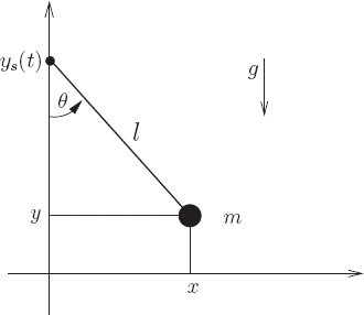
A pendulum driven at the pivot
Consider a pendulum (see figure 1.2) of length l and mass m, modeled as a point mass, supported by a pivot that is driven in the vertical direction by a given function of time ys.
The dimension of the configuration space for this system is one; we choose θ, shown in figure 1.2, as the generalized coordinate.
The position of the bob is given, in rectangular coordinates, by
The velocities are
obtained by differentiating along a path and abstracting to velocities at the moment.
The kinetic energy is
The potential energy is
A Lagrangian is L = T − V :
The Lagrangian is expressed as
(define ((T-pend m l g ys) local)
  (let ((t (time local))
        (theta (coordinate local))
        (thetadot (velocity local)))
    (let ((vys (D ys)))
      (* 1/2 m
         (+ (square (* l thetadot))
            (square (vys t))
            (* 2 l (vys t) thetadot (sin theta)))))))

(define ((V-pend m l g ys) local)
  (let ((t (time local))
        (theta (coordinate local)))
    (* m g (- (ys t) (* l (cos theta))))))

(define L-pend (- T-pend V-pend))
Lagrange's equation for this system is
(show-expression
  (((Lagrange-equations
      (L-pend 'm 'l 'g (literal-function 'y_s)))
    (literal-function 'theta))
't))Exercise 1.17: Bead on a helical wire
A bead of mass m is constrained to move on a frictionless helical wire. The helix is oriented so that its axis is horizontal. The diameter of the helix is d and its pitch (turns per unit length) is h. The system is in a uniform gravitational field with vertical acceleration g. Formulate a Lagrangian that describes the system and find the Lagrange equations of motion.
Exercise 1.18: Bead on a triaxial surface
A bead of mass m moves without friction on a triaxial ellipsoidal surface. In rectangular coordinates the surface satisfies
for some constants a, b, and c. Identify suitable generalized coordinates, formulate a Lagrangian, and find Lagrange's equations.
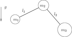
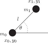
Exercise 1.19: Two-bar linkage
The two-bar linkage shown in figure 1.3 is constrained to move in the plane. It is composed of three small massive bodies interconnected by two massless rigid rods in a uniform gravitational field with vertical acceleration g. The rods are pinned to the central body by a hinge that allows the linkage to fold. The system is arranged so that the hinge is completely free: the members can go through all configurations without collision. Formulate a Lagrangian that describes the system and find the Lagrange equations of motion. Use the computer to do this, because the equations are rather big.
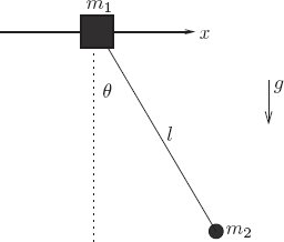
Exercise 1.20: Sliding pendulum
Consider a pendulum of length l attached to a support that is free to move horizontally, as shown in figure 1.4. Let the mass of the support be m1 and the mass of the pendulum bob be m2. Formulate a Lagrangian and derive Lagrange's equations for this system.
Why it works
In this section we show that L = T − V is in fact a suitable Lagrangian for rigidly constrained systems. We do this by requiring that the Lagrange equations be equivalent to the Newtonian vectorial dynamics with vector constraint forces.65
We consider a system of particles. The particle with index α has mass mα and position
that is, the distance between particles α and β is lαβ.
The Newtonian equation of motion for particle α says that the mass times the acceleration of particle α is equal to the sum of the potential forces and the constraint forces. The potential forces are derived as the negative gradient of the potential energy, and may depend on the positions of the other particles and the time. The constraint forces
where in the summation β ranges over only those particle indices for which there are rigid constraints with the particle indexed by α; we use the notation β ↔ α for the relation that there is a rigid constraint between the indicated particles.
The force of constraint is directed along the line between the particles, so we may write
where Fαβ(t) is the scalar magnitude of the tension in the constraint at time t. Note that
Formally, we can reproduce Newton's equations with the Lagrangian66
where the constraint forces are being treated as additional generalized coordinates. Here x is a structure composed of all the rectangular components xα of all the
but this is just a restatement of the constraints. The Lagrange equations for the coordinates of the particles are Newton's equations (1.91)
Now that we have a suitable Lagrangian, we can use the fact that Lagrangians can be reexpressed in any generalized coordinates to find a simpler Lagrangian. The strategy is to choose a new set of coordinates for which many of the coordinates are constants and the remaining coordinates are irredundant.
Let q be a tuple of generalized coordinates that specify the degrees of freedom of the system without redundancy. Let c be a tuple of other generalized coordinates that specify the distances between particles for which constraints are specified. The c coordinates will have constant values. The combination of q and c replaces the redundant rectangular coordinates x.67 In addition, we still have the F coordinates, which are the scalar constraint forces. Our new coordinates are the components of q, c, and F.
There exist functions fα that give the rectangular coordinates of the constituent particles in terms of q and c:
To reexpress the Lagrangian in terms of q, c, and F, we need to find vα in terms of the generalized velocities
Substituting these into Lagrangian (1.93), and using
we find
The Lagrange equations are derived by the usual procedure. Rather than write out all the gory details, let's think about how it will go.
The Lagrange equations associated with F just restate the constraints:
and consequently we know that along a solution path, c(t) = l and Dc(t) = D2c(t) = 0. We can use this result to simplify the Lagrange equations associated with q and c.
The Lagrange equations associated with q are the same as if they were derived from the Lagrangian68
but this is exactly T − V where T and V are computed from the generalized coordinates q, with fixed constraints. Notice that the constraint forces do not appear in the Lagrange equations for q because in the Lagrange equations they are multiplied by a term that is identically zero on the solution paths. So the Lagrange equations for T − V with irredundant generalized coordinates q and fixed constraints are equivalent to Newton's equations with vector constraint forces.
The Lagrange equations for c can be used to find the constraint forces. The Lagrange equations are a big mess so we will not show them explicitly, but in general they are equations in D2c, Dc, and c that will depend upon q, Dq, and F. The dependence on F is linear, so we can solve for F in terms of the solution path q and Dq, with c = l and Dc = D2c = 0.
If we are not interested in the constraint forces, we can abandon the full Lagrangian (1.99) in favor of Lagrangian (1.101), which is equivalent as far as the evolution of the generalized coordinates q is concerned.
The same derivation goes through even if the lengths lαβ specified in the interparticle distance constraints are a function of time. It can also be generalized to allow distance constraints to time-dependent positions, by making some of the positions of particles
Exercise 1.21: A dumbbell
In this exercise we will recapitulate the derivation of the Lagrangian for constrained systems for a particular simple system.
Consider two massive particles in the plane constrained by a massless rigid rod to remain a distance l apart, as in figure 1.5. There are apparently four degrees of freedom for two massive particles in the plane, but the rigid rod reduces this number to three.
We can uniquely specify the configuration with the redundant coordinates of the particles, say x0(t), y0(t) and x1(t), y1(t). The constraint (x1(t) − x0(t))2 + (y1(t) − y0(t))2 = l2 eliminates one degree of freedom.
a. Write Newton's equations for the balance of forces for the four rectangular coordinates of the two particles, given that the scalar tension in the rod is F.
b. Write the formal Lagrangian
such that Lagrange's equations will yield the Newton's equations you derived in part a.
c. Make a change of coordinates to a coordinate system with center of mass coordinates xCM, yCM, angle θ, distance between the particles c, and tension force F. Write the Lagrangian in these coordinates, and write the Lagrange equations.
d. You may deduce from one of these equations that c(t) = l. From this fact we get that Dc = 0 and D2c = 0. Substitute these into the Lagrange equations you just computed to get the equation of motion for xCM, yCM, θ.
e. Make a Lagrangian (= T − V) for the system described with the irredundant generalized coordinates xCM, yCM, θ and compute the Lagrange equations from this Lagrangian. They should be the same equations as you derived for the same coordinates in part d.
Exercise 1.22: Driven pendulum
Show that the Lagrangian (1.93) can be used to describe the driven pendulum (section 1.6.2), where the position of the pivot is a specified function of time: Derive the equations of motion using the Newtonian constraint force prescription, and show that they are the same as the Lagrange equations. Be sure to examine the equations for the constraint forces as well as the position of the pendulum bob.
Exercise 1.23: Fill in the details
Show that the Lagrange equations for Lagrangian (1.101) are the same as the Lagrange equations for Lagrangian (1.99) with the substitution c(t) = l, Dc(t) = D2c(t) = 0.
Exercise 1.24: Constraint forces
Find the tension in an undriven planar pendulum.
1.6.3 Constraints as Coordinate Transformations
The derivation of a Lagrangian for a constrained system involves steps that are analogous to those in the derivation of a coordinate transformation.
We can make a Lagrangian for the unconstrained system of particles in rectangular coordinates. In general there will be more coordinates than real degrees of freedom; the constraints will eliminate the redundancy. We then choose a convenient set of irredundant generalized coordinates that incorporate the constraints to describe our system. We express the redundant rectangular coordinates and velocities in terms of the irredundant generalized coordinates and generalized velocities, and we use these transformations to reexpress the Lagrangian in the generalized coordinates.
To carry out a coordinate transformation we specify how the configuration of a system expressed in one set of generalized coordinates can be reexpressed in terms of another set of generalized coordinates. We then determine the transformation of generalized velocities implied by the transformation of generalized coordinates. A Lagrangian that is expressed in terms of one of the sets of generalized coordinates can then be reexpressed in terms of the other set of generalized coordinates.
These are really two applications of the same process, so we can make Lagrangians for constrained systems by composing a Lagrangian for unconstrained particles with a coordinate transformation that incorporates the constraint. Our deduction that L = T − V is a suitable Lagrangian for a constrained systems was in fact based on a coordinate transformation from a set of coordinates subject to constraints to a set of irredundant coordinates plus constraint coordinates that are constant.
Let xα be the tuple of rectangular components of the constituent particle with index α, and let vα be its velocity. The Lagrangian
is the difference of kinetic and potential energies of the constituent particles. This is a suitable Lagrangian for a set of unconstrained free particles with potential energy V.
Let q be a tuple of irredundant generalized coordinates and v be the corresponding generalized velocity tuple. The coordinates q are related to xα, the coordinates of the constituent particles, by xα = fα(t, q), as before. The constraints among the constituent particles are taken into account in the definition of the fα. Here we view this as a coordinate transformation. What is unusual about this as a coordinate transformation is that the dimension of x is not the same as the dimension of q. From this coordinate transformation we can find the local-tuple transformation function (see section 1.6.1)
A Lagrangian for the constrained system can be obtained from the Lagrangian for the unconstrained system by composing it with the local-tuple transformation function from constrained coordinates to unconstrained coordinates:
The constraints enter only in the transformation.
To illustrate this we will find a Lagrangian for the driven pendulum introduced in section 1.6.2. As we saw on page 40, the T − V Lagrangian for a free particle of mass m in a vertical plane subject to a gravitational potential with acceleration g is
where y measures the height of the point mass. A program that computes this Lagrangian is
(define ((L-uniform-acceleration m g) local)
  (let ((q (coordinate local))
        (v (velocity local)))
    (let ((y (ref q 1)))
      (- (* 1/2 m (square v)) (* m g y)))))
The coordinate transformation from generalized coordinate θ to rectangular coordinates is x = l sin θ, y = ys(t) − l cos θ, where l is the length of the pendulum and ys gives the height of the support as a function of time. It is interesting that the drive enters only through the specification of the constraints. A program implementing this coordinate transformation is
(define ((dp-coordinates l y_s) local)
  (let ((t (time local))
        (theta (coordinate local)))
    (let ((x (* l (sin theta)))
          (y (- (y_s t) (* l (cos theta)))))
      (up x y))))
Using F->C we can deduce the local-tuple transformation and define the Lagrangian for the driven pendulum by composition:
(define (L-pend m l g y_s)
  (compose (L-uniform-acceleration m g)
           (F->C (dp-coordinates l y_s))))
The Lagrangian is
(show-expression
  ((L-pend 'm 'l 'g (literal-function 'y_s))
(up 't 'theta 'thetadot)))This is the same as the Lagrangian of equation (1.88) on page 51.
We have found a very interesting decomposition of the Lagrangian for constrained systems. One part consists of the difference of the kinetic and potential energy of the constituents. The other part describes the constraints that are specific to the configuration of a particular system.
Exercise 1.25: Foucault pendulum Lagrangian
A Foucault pendulum is a long-period pendulum of length l and mass m that is suspended at a height l above the surface of the Earth (radius R) at colatitude ϕ. If the pendulum is released, at rest, with nonzero displacement from the local vertical, it will oscillate in an apparent plane. However, the apparent plane of oscillation precesses as the Earth rotates. The Earth rotates with angular speed Ω.
One way to specify the position of the bob is to erect a Foucault pendulum at the North Pole and rotate it to a point on the surface of the Earth at the appropriate colatitude and a fixed longitude. Because the Earth is rotating this is a time-varying transformation. There are two parts of this transformation.
First, we relate the generalized coordinates θ and λ to the coordinates of the pendulum bob with the pendulum at the North pole. Let θ be the angle of the bob relative to the line through the center of the Earth and let λ be the precession angle. The rectangular coordinates of the bob for a pendulum at the North Pole are:
x0 = l sin θ cos λ
y0 = l sin θ sin λ
z0 = (R + l) − l cos θ.
Next, we rotate the pendulum to its actual location at colatitude ϕ. We can choose the longitude to be zero, so the angular position of the support of the bob is rotated by Ωt. The transformation of coordinates is:69
This second transformation can be implemented with the following code:
((compose (Rz (* 'Omega 't)) (Ry 'phi))
 (up 'x_0 'y_0 'z_0))
(up
  (+ (* x_0 (cos phi) (cos (* Omega t)))
     (* z_0 (sin phi) (cos (* Omega t)))
     (* -1 y_0 (sin (* Omega t))))
  (+ (* x_0 (cos phi) (sin (* Omega t)))
     (* z_0 (sin phi) (sin (* Omega t)))
     (* y_0 (cos (* Omega t))))
  (+ (* -1 x_0 (sin phi)) (* z_0 (cos phi))))
Construct a coordinate transformation F from these parts that you can use with F->C to compose with the free Lagrangian for a particle in a gravitational potential to make a Lagrangian for the Foucault pendulum. The Newtonian potential energy is −GMm/r, where r is the distance of the bob from the center of the Earth, and M is the mass of the Earth.
1.6.4 The Lagrangian Is Not Unique
Lagrangians are not in a one-to-one relationship with physical systems—many Lagrangians can be used to describe the same physical system. In this section we will demonstrate this by showing that the addition to the Lagrangian of a “total time derivative” of a function of the coordinates and time does not change the paths of stationary action or the equations of motion deduced from the action principle.
Total time derivatives
Let's first explain what we mean by a “total time derivative.” Let F be a function of time and coordinates. The function F on the path at time t is
So, by the chain rule
More formally, the time derivative of F along a path q is
Because F depends only on time and coordinates, we have
So we need only the first two components of DΓ[q],
to form the product
where
The function
is called the total time derivative of F ; it is a function of three arguments: the time, the generalized coordinates, and the generalized velocities.
In general, the total time derivative of a local-tuple function F is that function DtF that when composed with a local-tuple path is the time derivative of the composition of the function F with the same local-tuple path:
The total time derivative DtF is explicitly given by
where we take as many terms as needed to exhaust the arguments of F.
Exercise 1.26: Properties of Dt
The total time derivative DtF is not the derivative of the function F. Nevertheless, the total time derivative shares many properties with the derivative. Demonstrate that Dt has the following properties for local-tuple functions F and G, number c, and a function H with domain containing the range of G.
a. Dt(F + G) = DtF + DtG
b. Dt(cF) = cDtF
c. Dt(FG) = FDtG + (DtF)G
d. Dt(H ∘ G) = (DH ∘ G)DtG
Adding total time derivatives to Lagrangians
Consider two Lagrangians L and L′ that differ by the addition of a total time derivative of a function F that depends only on the time and the coordinates
The corresponding action integral is
The variational principle states that the action integral along a realizable trajectory is stationary with respect to variations of the trajectory that leave the configuration at the endpoints fixed. The action integrals S[q](t1, t2) and S′[q](t1, t2) differ by a term
that depends only on the coordinates and time at the endpoints and these are not allowed to vary. Thus, if S[q](t1, t2) is stationary for a path, then S′[q](t1, t2) will also be stationary. So either Lagrangian can be used to distinguish the realizable paths.
The addition of a total time derivative to a Lagrangian does not affect whether the action is stationary for a given path. So if we have two Lagrangians that differ by a total time derivative, the corresponding Lagrange equations are equivalent in that the same paths satisfy each. Moreover, the additional terms introduced into the action by the total time derivative appear only in the endpoint condition and thus do not affect the Lagrange equations derived from the variation of the action, so the Lagrange equations are the same. The Lagrange equations are not changed by the addition of a total time derivative to a Lagrangian.
Exercise 1.27: Lagrange equations for total time derivatives
Let F (t, q) be a function of t and q only, with total time derivative
Show explicitly that the Lagrange equations for DtF are identically zero, and thus that the addition of DtF to a Lagrangian does not affect the Lagrange equations.
The driven pendulum provides a nice illustration of adding total time derivatives to Lagrangians. The equation of motion for the driven pendulum (see section 1.6.2),
has an interesting and suggestive interpretation: it is the same as the equation of motion of an undriven pendulum, except that the acceleration of gravity g is augmented by the acceleration of the pivot D2ys. This intuitive interpretation was not apparent in the Lagrangian derived as the difference of the kinetic and potential energies in section 1.6.2. However, we can write an alternate Lagrangian with the same equation of motion that is as easy to interpret as the equation of motion:
With this Lagrangian it is apparent that the effect of the accelerating pivot is to modify the acceleration of gravity. Note, however, that it is not the difference of the kinetic and potential energies. Let's compare the two Lagrangians for the driven pendulum. The difference ΔL = L − L′ is
The two terms in ΔL that depend on neither θ nor
Properties of total time derivatives
If the local-tuple function G, with arguments (t, q, v), is the total time derivative of a function F, with arguments (t, q), then G must have certain properties.
From equation (1.112), we see that G must be linear in the generalized velocities
where neither G1 nor G0 depends on the generalized velocities: ∂2G1 = ∂2G0 = 0.
If G is the total time derivative of F then G1 = ∂1F and G0 = ∂0F, so
The partial derivative with respect to the time argument does not have structure, so ∂0∂1F = ∂1∂0F. So if G is the total time derivative of F then
Furthermore, G1 = ∂1F, so
If there is more than one degree of freedom these partials are actually structures of partial derivatives with respect to each coordinate. The partial derivatives with respect to two different coordinates must be the same independent of the order of the differentiation. So ∂1G1 must be symmetric.
Note that we have not shown that these conditions are sufficient for determining that a function is a total time derivative, only that they are necessary.
Exercise 1.28: Identifying total time derivatives
For each of the following functions, either show that it is not a total time derivative or produce a function from which it can be derived.
a. G(t, x, vx) = mvx
b. G(t, x, vx) = mvx cos t
c. G(t, x, vx) = vx cos t − x sin t
d. G(t, x, vx) = vx cos t + x sin t
e. G(t; x, y; vx, vy) = 2(xvx + yvy) cos t − (x2 + y2) sin t
f. G(t; x, y; vx, vy) = 2(xvx + yvy) cos t − (x2 + y2) sin t + y3vx + xvy
Exercise 1.29: Galilean invariance of kinetic energy
We have taken the kinetic energy of a set of particles indexed by α to be
a. Start with a Lagrangian for free particles, which is only the sum of their kinetic energies:
Carry out a coordinate transformation from old to new coordinates that consists of a shift and a uniform translation
Derive the Lagrangian in new coordinates.
b. The new Lagrangian can be put in the form
Thus the kinetic energy can be taken to be
1.7 Evolution of Dynamical State
Lagrange's equations are ordinary differential equations that the path must satisfy. They can be used to test if a proposed path is a realizable path of the system. However, we can also use them to develop a path, starting with initial conditions.
The state of a system is defined to be the information that must be specified for the subsequent evolution to be determined. Remember our juggler: he or she must throw the pin in a certain way for it to execute the desired motion. The juggler has control of the initial position and orientation of the pin, and the initial velocity and spin of the pin. Our experience with juggling and similar systems suggests that the initial configuration and the rate of change of the configuration are sufficient to determine the subsequent motion. Other systems may require higher derivatives of the configuration.
For Lagrangians that are written in terms of a set of generalized coordinates and velocities we have shown that Lagrange's equations are second-order ordinary differential equations. If the differential equations can be solved for the highest-order derivatives and if the differential equations satisfy the Lipschitz conditions,71 then there is a unique solution to the initial-value problem: given values of the solution and the lower derivatives of the solution at a particular moment, there is a unique solution function. Given irredundant coordinates the Lagrange equations satisfy these conditions.72 Thus a trajectory is determined by the generalized coordinates and the generalized velocities at any time. This is the information required to specify the dynamical state.
A complete local description of a path consists of the path and all of its derivatives at a moment. The complete local description of a path can be reconstructed from an initial segment of the local tuple, given a prescription for computing higher-order derivatives of the path in terms of lower-order derivatives. The state of the system is specified by that initial segment of the local tuple from which the rest of the complete local description can be deduced. The complete local description gives us the path near that moment. Actually, all we need is a rule for computing the next higher derivative; we can get all the rest from this. Assume that the state of a system is given by the tuple (t, q, v). If we are given a prescription for computing the acceleration a = A(t, q, v), then
and we have as a consequence
and so on. So the higher-derivative components of the local tuple are given by functions
First, we expand the Lagrange equations
so that the second derivative appears explicitly:
Solving this system for D2q, one obtains the generalized acceleration along a solution path q:
where [∂2∂2L ∘ Γ] is a structure that can be represented by a symmetric square matrix, so we can compute its inverse.73 The function that gives the acceleration is
where
That initial segment of the local tuple that specifies the state is called the local state tuple, or, more simply, the state tuple.74
We can express the function that gives the acceleration as a function of the state tuple as the following procedure. It takes a procedure that computes the Lagrangian, and returns a procedure that takes a state tuple as its argument and returns the acceleration.75
(define (Lagrangian->acceleration L)
  (let ((P ((partial 2) L)) (F ((partial 1) L)))
    (solve-linear-left
      ((partial 2) P)
      (- F
         (+ ((partial 0) P)
            (* ((partial 1) P) velocity))))))
Once we have a way of computing the acceleration from the coordinates and the velocities, we can give a prescription for computing the derivative of the state as a function of the state. For the state (t, q(t), Dq(t)) at the moment t the derivative of the state is (1, Dq(t), D2q(t)) = (1, Dq(t), A(t, q(t), Dq(t))). The procedure Lagrangian->state-derivative takes a Lagrangian and returns a procedure that takes a state and returns the derivative of the state:
(define (Lagrangian->state-derivative L)
  (let ((acceleration (Lagrangian->acceleration L)))
    (lambda (state)
      (up 1
          (velocity state)
          (acceleration state)))))
We represent a state by an up tuple of the components of that initial segment of the local tuple that determine the state.
For example, the parametric state derivative for a harmonic oscillator is
(define (harmonic-state-derivative m k)
  (Lagrangian->state-derivative (L-harmonic m k)))

((harmonic-state-derivative 'm 'k)
 (up 't (up 'x 'y) (up 'v_x 'v_y)))
(up 1 (up v_x v_y) (up (/ (* -1 k x) m) (/ (* -1 k y) m)))
The Lagrange equations are a second-order system of differential equations that constrain realizable paths q. We can use the state derivative to express the Lagrange equations as a first-order system of differential equations that constrain realizable coordinate paths q and velocity paths v:
(define ((Lagrange-equations-first-order L) q v)
  (let ((state-path (qv->state-path q v)))
    (- (D state-path)
       (compose (Lagrangian->state-derivative L)
                state-path))))

(define ((qv->state-path q v) t)
  (up t (q t) (v t)))
For example, we can find the first-order form of the equations of motion of a two-dimensional harmonic oscillator:
(show-expression
  (((Lagrange-equations-first-order (L-harmonic 'm 'k))
    (up (literal-function 'x)
        (literal-function 'y))
    (up (literal-function 'v_x)
        (literal-function 'v_y)))
   't))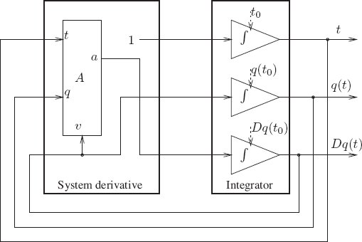
The zero in the first element of the structure of the Lagrange equations residuals is just the tautology that time advances uniformly: the time function is just the identity, so its derivative is one and the residual is zero. The equations in the second element constrain the velocity path to be the derivative of the coordinate path. The equations in the third element give the rate of change of the velocity in terms of the applied forces.
Numerical integration
A set of first-order ordinary differential equations that give the state derivative in terms of the state can be integrated to find the state path that emanates from a given initial state. Numerical integrators find approximate solutions of such differential equations by a process illustrated in figure 1.6. The state derivative produced by Lagrangian->state-derivative can be used by a package that numerically integrates systems of first-order ordinary differential equations.
The procedure state-advancer can be used to find the state of a system at a specified time, given an initial state, which includes the initial time, and a parametric state-derivative procedure.76 For example, to advance the state of a two-dimensional harmonic oscillator we write77
((state-advancer harmonic-state-derivative 2.0 1.0)
 (up 1.0 (up 1.0 2.0) (up 3.0 4.0))
 10.0
 1.0e-12)
(up 11.0
    (up 3.7127916645844437 5.420620823651583)
    (up 1.6148030925459782 1.8189103724750855))
The arguments to state-advancer are a parametric state derivative, harmonic-state-derivative, and the state-derivative parameters (mass 2 and spring constant 1). A procedure is returned that takes an initial state, (up 1 (up 1 2) (up 3 4)); a time increment, 10; and a relative error tolerance, 1.0e-12. The output is an approximation to the state at the specified final time.
Consider the driven pendulum described in section 1.6.2 with a periodic drive. We choose ys(t) = A cos ωt.
(define ((periodic-drive amplitude frequency phase) t)
  (* amplitude (cos (+ (* frequency t) phase))))

(define (L-periodically-driven-pendulum m l g A omega)
  (let ((ys (periodic-drive A omega 0)))
    (L-pend m l g ys)))
Lagrange's equation for this system is
(show-expression
  (((Lagrange-equations
      (L-periodically-driven-pendulum 'm 'l 'g 'A 'omega))
    (literal-function 'theta))
't))The parametric state derivative for the periodically driven pendulum is
(define (pend-state-derivative m l g A omega)
  (Lagrangian->state-derivative
    (L-periodically-driven-pendulum m l g A omega)))

(show-expression
  ((pend-state-derivative 'm 'l 'g 'A 'omega)
(up 't 'theta 'thetadot)))To examine the evolution of the driven pendulum we need a mechanism that evolves a system for some interval while monitoring aspects of the system as it evolves. The procedure evolve provides this service, using state-advancer repeatedly to advance the state to the required moments. The procedure evolve takes a parametric state derivative and its parameters and returns a procedure that evolves the system from a specified initial state to a number of other times, monitoring some aspect of the state at those times. To generate a plot of the angle versus time we make a monitor procedure that generates the plot as the evolution proceeds:78
(define ((monitor-theta win) state)
  (let ((theta ((principal-value :pi) (coordinate state))))
    (plot-point win (time state) theta)))

(define plot-win (frame 0.0 100.0 :-pi :pi))

((evolve pend-state-derivative
         1.0 ;m=1kg
         1.0 ;l=1m
         9.8 ;g=9.8m/s^2
         0.1 ;a=1/10 m
         (* 2.0 (sqrt 9.8)) ) ;omega
 (up 0.0 ;t0=0
     1.0 ;theta0=1 radian
     0.0) ;thetadot0=0 radians/s
 (monitor-theta plot-win)
 0.01 ;step between plotted points
 100.0 ;final time
 1.0e-13) ;local error tolerance
Figure 1.7 shows the angle θ versus time for a couple of orbits for the driven pendulum. The initial conditions for the two runs are the same except that in one the bob is given a tiny velocity equal to 10−10m/s, about one atom width per second. The initial segments of the two orbits are indistinguishable. After about 75 seconds the two orbits diverge and become completely different. This extreme sensitivity to tiny changes in initial conditions is characteristic of what is called chaotic behavior. Later, we will investigate this example further, using other tools such as Lyapunov exponents, phase space, and Poincaré sections.
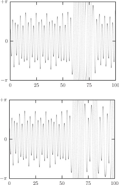
Exercise 1.30: Orbits in a central potential
A Lagrangian for planar motion of a particle of mass m in a central field with potential energy V (r) = −βrα is
a. Write a program to evolve the motion of a particle subject to this Lagrangian and display the orbit in the plane.
b. Evolve this system with α = +2 (harmonic oscillator). Observe that it describes an ellipse with its center at the origin, for a wide variety of initial conditions.
c. Evolve this system with α = −1 (Newtonian gravity). Observe that it describes an ellipse with a focus at the origin, for a wide variety of initial conditions.
d. Evolve this system with α = +1/4. Observe that it describes a trefoil with its center at the origin.
Exercise 1.31: Foucault pendulum evolution
If a Foucault pendulum is erected at the North Pole, it will precess exactly once in a day. If it is erected at the Equator it will not precess at all. It is widely reported that the precession rate is proportional to the cosine of the colatitude.
a. Evolve the Foucault pendulum, using the Lagrangian you constructed in exercise 1.25 on page 62. You should look at the precession angle λ as a function of time.
b. How does the rate of precession compare to the predicted rate? You should expect to see an error caused by the fact that the local vertical, as defined by a plumb bob, is not directed to the center of the Earth.
c. Let Δϕ be the angle between the local vertical and the direction to the center of the Earth. How does the precession rate compare to the predicted precession rate with the colatitude corrected to ϕ − Δϕ? Is this perfect?
1.8 Conserved Quantities
A function of the state of the system that is constant along a solution path is called a conserved quantity or a constant of motion.79 If C is a conserved quantity, then
for solution paths q. In this section, we will investigate systems with symmetry and find that symmetries are associated with conserved quantities. For instance, linear momentum is conserved in a system with translational symmetry, angular momentum is conserved if there is rotational symmetry, energy is conserved if the system does not depend on the origin of time. We first consider systems for which a coordinate system can be chosen that expresses the symmetry naturally, and later discuss systems for which no coordinate system can be chosen that simultaneously expresses all symmetries.
1.8.1 Conserved Momenta
If a Lagrangian L(t, q, v) does not depend on some particular coordinate qi, then
and the corresponding ith component of the Lagrange equations is
The derivative of a component is equal to the component of the derivative, so this is the same as
and we can see that
is a conserved quantity. The function
Given the coordinate path q and the Lagrangian L, the momentum path p is
with components
The momentum path is well defined for any path q. If the path is realizable and the Lagrangian does not depend on qi, then pi is a constant function
The constant value of pi may be different for different trajectories.
Examples of conserved momenta
The free-particle Lagrangian
For a particle in a central force field (section 1.6), the Lagrangian
depends on r but is independent of φ. The momentum state function is
It has two components. The first component, the “radial momentum,” is not conserved. The second component, the “angular momentum,” is conserved along any solution trajectory.
If the central-potential problem had been expressed in rectangular coordinates, then all of the coordinates would have appeared in the Lagrangian. In that case there would not be any obvious conserved quantities. Nevertheless, the motion of the system does not depend on the choice of coordinates, so the angular momentum is still conserved.
We see that there is great advantage in making a judicious choice for the coordinate system. If we can choose the coordinates so that a symmetry of the system is reflected in the Lagrangian by the absence of some coordinate component, then the existence of a corresponding conserved quantity will be evident.82
1.8.2 Energy Conservation
Momenta are conserved by the motion if the Lagrangian does not depend on the corresponding coordinate. There is another constant of the motion, the energy, if the Lagrangian
Consider the time derivative of the Lagrangian along a solution path q:
Using Lagrange's equations to rewrite the second term yields
Isolating ∂0L and combining the other terms we get
where, as before,
is conserved along realizable paths. The function ℰ is called the energy state function.83 The energy state function for a system depends on the choice of Lagrangian used to describe the system.84 Let E = ℰ ∘ Γ[q] denote the energy function on the path q. The energy function has a constant value along any realizable trajectory if the Lagrangian has no explicit time dependence; the energy E may have a different value for different trajectories. A system that has no explicit time dependence is called autonomous.
Given a Lagrangian procedure L, we may construct the energy function:
(define (Lagrangian->energy L)
  (let ((P ((partial 2) L)))
    (- (* P velocity) L)))
Energy in terms of kinetic and potential energies
In some cases the energy can be written as the sum of kinetic and potential energies. Suppose the system is composed of particles with rectangular coordinates xα, the movement of which may be subject to constraints, and that these rectangular coordinates are some functions of the generalized coordinates q and possibly time t: xα = fα(t, q). We form the Lagrangian as L = T − V and compute the kinetic energy in terms of q by writing the rectangular velocities in terms of the generalized velocities:
The kinetic energy is
where vα is the magnitude of vα.
If the fα functions do not depend explicitly on time (∂0fα = 0), then the rectangular velocities are homogeneous functions of the generalized velocities of degree 1, and T is a homogeneous function of the generalized velocities of degree 2, because it is formed by summing the square of homogeneous functions of degree 1. If T is a homogeneous function of degree 2 in the generalized velocities then
where the second equality follows from Euler's theorem on homogeneous functions.85 The energy state function is
So if fα is independent of time, the energy function can be rewritten
Notice that if V depends on time the energy is still the sum of the kinetic energy and potential energy, but the energy is not conserved.
The energy state function is always well defined, whether or not it can be written in the form T + V, and whether or not it is conserved along realizable paths.
Exercise 1.32: Time-dependent constraints
An analogous result holds when the fα depend explicitly on time.
a. Show that in this case the kinetic energy contains terms that are linear in the generalized velocities.
b. By adding a total time derivative, show that the Lagrangian can be written in the form L = A − B, where A is a homogeneous quadratic form in the generalized velocities and B is independent of velocity.
c. Show, using Euler's theorem, that the energy function is ℰ = A+B.
An example in which terms that were linear in the velocity were removed from the Lagrangian by adding a total time derivative has already been given: the driven pendulum.
Exercise 1.33: Falling off a log
A particle of mass m slides off a horizontal cylinder of radius R in a uniform gravitational field with acceleration g. If the particle starts close to the top of the cylinder with zero initial speed, with what angular velocity does it leave the cylinder? Use the method of incorporating constraint forces that we introduced in section 1.6.2, together with conservation of energy.
1.8.3 Central Forces in Three Dimensions
One important physical system is the motion of a particle in a central field in three dimensions, with an arbitrary potential energy V (r) depending only on the radius. We will describe this system in spherical coordinates r, θ, and φ, where θ is the colatitude and φ is the longitude. The kinetic energy has three terms:
As a procedure:
(define ((T3-spherical m) state)
  (let ((q (coordinate state))
        (qdot (velocity state)))
    (let ((r (ref q 0))
          (theta (ref q 1))
          (rdot (ref qdot 0))
          (thetadot (ref qdot 1))
          (phidot (ref qdot 2)))
      (* 1/2 m
         (+ (square rdot)
            (square (* r thetadot))
            (square (* r (sin theta) phidot)))))))
A Lagrangian is then formed by subtracting the potential energy:
(define (L3-central m Vr)
  (define (Vs state)
    (let ((r (ref (coordinate state) 0)))
      (Vr r)))
  (- (T3-spherical m) Vs))
Let's first look at the generalized forces (the derivatives of the Lagrangian with respect to the generalized coordinates). We compute these with a partial derivative with respect to the coordinate argument of the Lagrangian:
(show-expression
  (((partial 1) (L3-central 'm (literal-function 'V)))
   (up 't
       (up 'r 'theta 'phi)
(up 'rdot 'thetadot 'phidot))))The φ component of the force is zero because φ does not appear in the Lagrangian (it is a cyclic coordinate). The corresponding momentum component is conserved. Compute the momenta:
(show-expression
  (((partial 2) (L3-central 'm (literal-function 'V)))
   (up 't
       (up 'r 'theta 'phi)
(up 'rdot 'thetadot 'phidot))))The momentum conjugate to φ is conserved. This is the z component of the angular momentum
(define ((ang-mom-z m) rectangular-state)
  (let ((xyz (coordinate rectangular-state))
        (v (velocity rectangular-state)))
    (ref (cross-product xyz (* m v)) 2)))

(define (s->r spherical-state)
  (let ((q (coordinate spherical-state)))
    (let ((r (ref q 0))
          (theta (ref q 1))
          (phi (ref q 2)))
      (let ((x (* r (sin theta) (cos phi)))
            (y (* r (sin theta) (sin phi)))
            (z (* r (cos theta))))
(up x y z)))))(show-expression
((compose (ang-mom-z 'm) (F->C s->r))
(up 't
(up 'r 'theta 'phi)
(up 'rdot 'thetadot 'phidot))))The choice of the z-axis is arbitrary, so the conservation of any component of the angular momentum implies the conservation of all components. Thus the total angular momentum is conserved. We can choose the z-axis so all of the angular momentum is in the z component. Since
We can also see that the energy state function computed from the Lagrangian for a central field is in fact T + V :
(show-expression
  ((Lagrangian->energy (L3-central 'm (literal-function 'V)))
   (up 't
       (up 'r 'theta 'phi)
(up 'rdot 'thetadot 'phidot))))The energy is conserved because the Lagrangian has no explicit time dependence.
Exercise 1.34: Driven spherical pendulum
A spherical pendulum is a massive bob, subject to uniform gravity, that may swing in three dimensions, but remains at a given distance from the pivot. Formulate a Lagrangian for a spherical pendulum driven by vertical motion of the pivot. What symmetry(ies) can you find? Find coordinates that express the symmetry(ies). What is conserved? Give analytic expression(s) for the conserved quantity(ies).
1.8.4 The Restricted Three-Body Problem
Consider the situation of two bodies of masses M0 and M1 in circular orbit about their common center of mass. What is the behavior of a third particle, gravitationally attracted to the other two, that must move in the plane of their circular orbit? Assume that the third particle has such small mass that we can neglect its effect on the orbits of the two massive particles.
The third particle, of mass m, moves in a field derived from a time-varying gravitational potential energy. We have:
(define ((L0 m V) local)
  (let ((t (time local))
        (q (coordinates local))
        (v (velocities local)))
    (- (* 1/2 m (square v)) (V t q))))
Let a be the constant distance between the two bodies. If we put the center of mass at the origin of the coordinate system then the distances of the two particles from the origin are:
Each massive particle revolves in a circle about their common center of mass with angular frequency Ω. The radii of the circles are the distances given above. Kepler's law gives the angular frequency of the orbit:
We choose our axes so that at t = 0 the body with mass M1 is on the positive
(define ((V a GM0 GM1 m) t xy)
  (let ((Omega (sqrt (/ (+ GM0 GM1) (expt a 3))))
        (a0 (* (/ GM1 (+ GM0 GM1)) a))
        (a1 (* (/ GM0 (+ GM0 GM1)) a)))
    (let ((x (ref xy 0)) (y (ref xy 1))
                         (x0 (* -1 a0 (cos (* Omega t))))
                         (y0 (* -1 a0 (sin (* Omega t))))
                         (x1 (* +1 a1 (cos (* Omega t))))
                         (y1 (* +1 a1 (sin (* Omega t)))))
      (let ((r0
              (sqrt (+ (square (- x x0)) (square (- y y0)))))
            (r1
              (sqrt (+ (square (- x x1)) (square (- y y1))))))
        (- (+ (/ (* GM0 m) r0) (/ (* GM1 m) r1)))))))
It is convenient to examine the motion of the third particle in a rotating coordinate system where the massive particles are fixed. We can place the rotating axes so that the two massive particles are on the
where now
(define ((LR3B m a GM0 GM1) local)
  (let ((q (coordinates local))
        (qdot (velocities local))
        (Omega (sqrt (/ (+ GM0 GM1) (expt a 3))))
        (a0 (* (/ GM1 (+ GM0 GM1)) a))
        (a1 (* (/ GM0 (+ GM0 GM1)) a)))
    (let ((x (ref q 0))     (y (ref q 1))
                            (xdot (ref qdot 0)) (ydot (ref qdot 1)))
      (let ((r0 (sqrt (+ (square (+ x a0)) (square y))))
            (r1 (sqrt (+ (square (- x a1)) (square y)))))
        (+ (* 1/2 m (square qdot))
           (* 1/2 m (square Omega) (square q))
           (* m Omega (- (* x ydot) (* xdot y)))
           (/ (* GM0 m) r0) (/ (* GM1 m) r1))))))
Notice that the Lagrangian in rotating coordinates is independent of time. So the energy state function defined by this Lagrangian is a conserved quantity. Let's compute it. It is clearest if we express the result in terms of Ω, a0, and a1, so we make those into explicit parameters of the Lagrangian:
(define ((LR3B1 m a0 a1 Omega GM0 GM1) local)
  (let ((q (coordinates local))
        (qdot (velocities local)))
    (let ((x (ref q 0))     (y (ref q 1))
                            (xdot (ref qdot 0)) (ydot (ref qdot 1)))
      (let ((r0 (sqrt (+ (square (+ x a0)) (square y))))
            (r1 (sqrt (+ (square (- x a1)) (square y)))))
        (+ (* 1/2 m (square qdot))
           (* 1/2 m (square Omega) (square q))
           (* m Omega (- (* x ydot) (* xdot y)))
           (/ (* GM0 m) r0) (/ (* GM1 m) r1))))))
And we compute the energy state function (with a bit of hand simplification):
((Lagrangian->energy (LR3B1 'm 'a_0 'a_1 'Omega 'GM_0 'GM_1))
 (up 't (up 'x_r 'y_r) (up 'v_r^x 'v_r^y)))
(+ (* 1/2 m (expt v_r^x 2))
   (* 1/2 m (expt v_r^y 2))
   (/ (* -1 GM_0 m)
      (sqrt (+ (expt (+ x_r a_0) 2) (expt y_r 2))))
   (/ (* -1 GM_1 m)
      (sqrt (+ (expt (- x_r a_1) 2) (expt y_r 2))))
   (* -1/2 m (expt Omega 2) (expt x_r 2))
   (* -1/2 m (expt Omega 2) (expt y_r 2)))
If we separate this into a velocity-dependent part and a velocity-independent part we get
where
This constant of motion of the restricted three-body problem is called the Jacobi constant.86 Notice that the energy function is a positive definite quadratic form in the components of the velocity (in rotating coordinates) plus a function that depends only on the rotating coordinates. Note that the energy state function does not have terms that are linear in the velocities
Exercise 1.35: Restricted equations of motion
Derive the Lagrange equations for the restricted three-body problem, given the Lagrangian (1.150). Identify the Coriolis and centrifugal force terms in your equations of motion.
1.8.5 Noether's Theorem
We have seen that if a system has a symmetry and a coordinate system can be chosen so that the Lagrangian does not depend on the coordinate associated with that symmetry, then there is a conserved quantity associated with the symmetry. However, there are more general symmetries that no coordinate system can fully express. For example, motion in a central potential is spherically symmetric (the dynamical system is invariant under rotations about any axis), but the expression of the Lagrangian for the system in spherical coordinates exhibits symmetry around only one axis. More generally, a Lagrangian has a symmetry if there is a coordinate transformation that leaves the Lagrangian unchanged. A continuous symmetry is a parametric family of symmetries. Noether proved that for any continuous symmetry there is a conserved quantity.
Consider a parametric coordinate transformation
To this parametric coordinate transformation there corresponds a parametric state transformation
We require that the transformation
for any s. The Lagrangian L is the same function as the transformed Lagrangian
That
where we have rewritten the velocity component of
where we have used the fact that87
On a realizable path q we can use the Lagrange equations to rewrite the first term of equation (1.157):
For s = 0 the paths q and q′ are the same, because
Thus the state function
is conserved along solution trajectories. This conserved quantity is called Noether's integral. It is the product of the momentum and a vector associated with the symmetry.
Illustration: motion in a central potential
For example, consider the central-potential Lagrangian in rectangular coordinates:
and a parametric rotation Rz(s) about the z axis
The rotation is an orthogonal transformation so
Differentiating along a path, we get
so the velocities also transform by an orthogonal transformation, and
and we see that L′ is precisely the same function as L.
The momenta are
and
So the Noether integral is
which we recognize as minus the z component of the angular momentum:
The procedure calls ((Rx angle-x) q), ((Ry angle-y) q), and ((Rz angle-z) q) rotate the rectangular tuple q about the indicated axis by the indicated angle.88 We use these to make a parametric coordinate transformation F-tilde:
(define (F-tilde angle-x angle-y angle-z)
  (compose (Rx angle-x) (Ry angle-y) (Rz angle-z) coordinate))
A Lagrangian for motion in a central potential is
(define ((L-central-rectangular m U) state)
  (let ((q (coordinate state))
        (v (velocity state)))
    (- (* 1/2 m (square v))
       (U (sqrt (square q))))))
The Noether integral is then
(define the-Noether-integral
  (let ((L (L-central-rectangular
             'm (literal-function 'U))))
    (* ((partial 2) L) ((D F-tilde) 0 0 0))))

(the-Noether-integral
  (up 't
      (up 'x 'y 'z)
      (up 'vx 'vy 'vz)))
(down (+ (* m vy z) (* -1 m vz y))
      (+ (* m vz x) (* -1 m vx z))
      (+ (* m vx y) (* -1 m vy x)))
We get all three components of the angular momentum.
Exercise 1.36: Noether integral
Consider motion on an ellipsoidal surface. The surface is specified by:
Formulate a Lagrangian for frictionless motion on this surface. Assume that two of the axes of the ellipsoid are equal: b = c.
Using angular coordinates (θ, ϕ), where θ is colatitude from the ẑ-axis, and ϕ is longitude measured from the
Note that the choice of coordinates does not build in this symmetry.
1.9 Abstraction of Path Functions
An essential step in the derivation of the local-tuple transformation function C from the coordinate transformation F was the deduction of the relationship between the velocities in the two coordinate systems. We did this by inserting coordinate paths into the coordinate transformation function F, differentiating, and then generalizing the results on the path to arbitrary velocities at a moment. The last step is an example of a more general problem of abstracting a local-tuple function from a path function. Given a function f of a local tuple, a corresponding path-dependent function
Two paths that have the same local description up to the nth derivative are said to osculate with order n contact. For example, a path and the truncated power series representation of the path up to order n have order n contact; if fewer than n derivatives are needed by a local-tuple function, the path and the truncated power series representation are equivalent. Let O be a function that generates an osculating path with the given local-tuple components. So O(t, q, v, …)(t) = q, D(O(t, q, v, …))(t) = v, and in general
The number of components of the local tuple that are required is finite, but unspecified. One way of constructing O is through the truncated power series
where the number of terms is the same as the number of components of the local tuple that are specified.
Given the path function
Let
From equation (1.172) we see that
The procedure Gamma-bar implements the function
(define ((Gamma-bar f-bar) local)
  ((f-bar (osculating-path local)) (time local)))
The procedure osculating-path takes a number of local components and returns a path with these components; it is implemented as a power series.
We can use Gamma-bar to construct the procedure F->C that takes a coordinate transformation F and generates the procedure that transforms local tuples. The procedure F->C constructs a path-dependent procedure f-bar that takes a coordinate path in the primed system and returns the local tuple of the corresponding path in the unprimed coordinate system. It then uses Gamma-bar to abstract f-bar to arbitrary local tuples in the primed coordinate system.90
(define (F->C F)
  (define (C local)
    (let ((n (vector-length local)))
      (define (f-bar q-prime)
        (define q
          (compose F (Gamma q-prime)))
        (Gamma q n))
      ((Gamma-bar f-bar) local)))
  C)

(show-expression
  ((F->C p->r)
(up 't (up 'r 'theta) (up 'rdot 'thetadot))))Notice that in this definition of F->C we do not explicitly calculate any derivatives. The calculation that led up to the state transformation (1.77) is not needed.
We can also use
The total time derivative can be expressed as a program:
(define (Dt F)
  (define (DtF state)
    (let ((n (vector-length state)))
      (define (DF-on-path q)
        (D (compose F (Gamma q (- n 1)))))
      ((Gamma-bar DF-on-path) state)))
  DtF)
Given a procedure F implementing a local-tuple function and a path q, we construct a new procedure (compose F (Gamma q)). The procedure DF-on-path implements the derivative of this function of time. We then abstract this off the path with Gamma-bar to give the total time derivative.
Exercise 1.37: Velocity transformation
Use the procedure Gamma-bar to construct a procedure that transforms velocities given a coordinate transformation. Apply this procedure to the procedure p->r to deduce (again) equation (1.67) on page 42.
Lagrange equations at a moment
Given a Lagrangian, the Lagrange equations test paths to determine whether they are realizable paths of the system. The Lagrange equations relate the path and its derivatives. The fact that the Lagrange equations must be satisfied at each moment suggests that we can abstract the Lagrange equations off the path and write them as relations among the local-tuple components of realizable paths.
Let
Realizable paths q satisfy the Lagrange equations
The path-dependent Lagrange equations can be converted to local Lagrange equations using
The operator
The Euler–Lagrange operator is explicitly
The procedure Euler-Lagrange-operator implements
(define (Euler-Lagrange-operator L)
  (- (Dt ((partial 2) L)) ((partial 1) L))).
For example, applied to the Lagrangian for the harmonic oscillator, we have
((Euler-Lagrange-operator
   (L-harmonic 'm 'k))
 (up 't 'x 'v 'a))
(+ (* a m) (* k x))
Notice that the components of the local tuple are individually specified. Using equation (1.179), the Lagrange equations for the harmonic oscillator are
((compose
   (Euler-Lagrange-operator (L-harmonic 'm 'k))
   (Gamma (literal-function 'x) 4))
 't)
(+ (* k (x t)) (* m (((expt D 2) x) t)))
Exercise 1.38: Properties of E
Let F and G be two Lagrangian-like functions of a local tuple, C be a local-tuple transformation function, and c a constant. Demonstrate the following properties:
a.
b.
c.
d.
1.10 Constrained Motion
An advantage of the Lagrangian approach is that coordinates can often be chosen that exactly describe the freedom of the system, automatically incorporating any constraints. We may also use coordinates that have more freedom than the system actually has and consider explicit constraints among the coordinates. For example, the planar pendulum has a one-dimensional configuration space. We have formulated this problem using the angle from the vertical as the configuration coordinate. Alternatively, we may choose to represent the pendulum as a body moving in the plane, constrained to be on the circle of the correct radius around the pivot. We would like to have valid descriptions for both choices and show they are equivalent. In this section we develop tools to handle problems with explicit constraints. The constraints considered here are more general than those used in the demonstration that the Lagrangian for systems with rigid constraints can be written as the difference of kinetic and potential energies (see section 1.6.2).
Suppose the configuration of a system with n degrees of freedom is specified by n + 1 coordinates and that configuration paths q are constrained to satisfy some relation of the form
How do we formulate the equations of motion? One approach would be to use the constraint equation to eliminate one of the coordinates in favor of the rest; then the evolution of the reduced set of generalized coordinates would be described by the usual Lagrange equations. The equations governing the evolution of coordinates that are not fully independent should be equivalent.
We can address the problem of formulating equations of motion for systems with redundant coordinates by returning to the action principle. Realizable paths are distinguished from other paths by having stationary action. Stationary refers to the fact that the action does not change with certain small variations of the path. What variations should be considered? We have seen that velocity-independent rigid constraints can be used to eliminate redundant coordinates. In the irredundant coordinates we distinguished realizable paths by using variations that by construction satisfy the constraints. Thus in the case where constraints can be used to eliminate redundant coordinates we can restrict the variations in the path to those that are consistent with the constraints.
So how does the restriction of the possible variations affect the argument that led to Lagrange's equations (refer to section 1.5)? Actually most of the calculation is unaffected. The condition that the action is stationary still reduces to the conditions (1.17) or (1.34):
At this point we argued that because the variations η are arbitrary (except for conditions at the endpoints), the only way for the integral to be zero is for the integrand to be zero. Furthermore, the freedom in our choice of η allowed us to deduce that the factor multiplying η in the integrand must be identically zero, thereby deriving Lagrange's equations.
Now the choice of η is not completely free. We can still deduce from the arbitrariness of η that the integrand must be zero,91 but we can no longer deduce that the factor multiplying η is zero (only that the projection of this factor onto acceptable variations is zero). So we have
with η subject to the constraints.
A path q satisfies the constraint if
We can say that the variation must be “tangent” to the constraint surface. Expanding this with the chain rule, a variation η is tangent to the constraint surface φ if
Note that these are functions of time; the variation at a given time is tangent to the constraint at that time.
1.10.1 Coordinate Constraints
Consider constraints that do not depend on velocities:
In this case the variation is tangent to the constraint surface if
Together, equations (1.183) and (1.186) should determine the motion, but how do we eliminate η? The residual of the Lagrange equations is orthogonal92 to any η that is orthogonal to the normal to the constraint surface. A vector that is orthogonal to all vectors orthogonal to a given vector is parallel to the given vector. Thus, the residual of Lagrange's equations is parallel to the normal to the constraint surface; the two must be proportional:
That the two vectors are parallel everywhere along the path does not guarantee that the proportionality factor is the same at each moment along the path, so the proportionality factor λ is some function of time, which may depend on the path under consideration. These equations, with the constraint equation φ ∘ Γ[q] = 0, are the governing equations. These equations are sufficient to determine the path q and to eliminate the unknown function λ.
Now watch this
Suppose we form an augmented Lagrangian by treating λ as one of the coordinates:
The Lagrange equations associated with the coordinates q are just the modified Lagrange equations (1.187), and the Lagrange equation associated with λ is just the constraint equation. (Note that
Alternatively
How do we know that we have enough information to eliminate the unknown function λ from equations (1.187), or that the extra degree of freedom introduced in Lagrangian (1.188) is purely formal?
If λ can be written as a composition of a state-dependent function with the path: λ = Λ ∘ Γ[q] then it is redundant as a degree of freedom. Consider the Lagrangian
This new Lagrangian has no extra degrees of freedom. The Lagrange equations for L″ are the Lagrange equations for L with additional terms arising from the product Λφ. Applying the Euler–Lagrange operator
Composition of
where we have used λ = Λ ∘ Γ[q]. If we now use the fact that we are dealing only with coordinate constraints, ∂2φ = 0, then
The Lagrange equations are the same as those derived from the augmented Lagrangian L′. The difference is that now we see that λ = Λ ∘ Γ[q] is determined by the unaugmented state. This is the same as saying that λ can be eliminated.
Considering only the formal validity of the Lagrange equations for the augmented Lagrangian, we could not deduce that λ could be written as the composition of a state-dependent function Λ with Γ[q]. The explicit Lagrange equations derived from the augmented Lagrangian depend on the accelerations D2q as well as λ, so we cannot deduce separately that either is the composition of a state-dependent function and Γ[q]. However, now we see that λ is such a composition. This allows us to deduce that D2q is also a state-dependent function composed with the path. The evolution of the system is determined from the dynamical state.
The pendulum using constraints
The pendulum can be formulated as the motion of a massive particle in a vertical plane subject to the constraint that the distance to the pivot is constant (see figure 1.8).
In this formulation, the kinetic and potential energies in the Lagrangian are those of an unconstrained particle in a uniform gravitational acceleration. A Lagrangian for the unconstrained particle is
The constraint that the pendulum moves in a circle of radius l about the pivot is94
The augmented Lagrangian is
The Lagrange equations for the augmented Lagrangian are
These equations are sufficient to solve for the motion of the pendulum.
It should not be surprising that these equations simplify if we switch to “polar” coordinates
Substituting this into the constraint equation, we determine that r = l, a constant. Forming the derivatives and substituting into the other two equations, we find
Multiplying the first by cos θ and the second by sin θ and adding, we find
which we recognize as the correct equation for the pendulum. This is the same as the Lagrange equation for the pendulum using the unconstrained generalized coordinate θ. For completeness, we can find λ in terms of the other variables:
This confirms that λ is really the composition of a function of the state with the state path. Notice that 2lλ is a force—it is the sum of the outward component of the gravitational force and the centrifugal force. Using this interpretation in the two coordinate equations of motion, we see that the terms involving λ are the forces that must be applied to the unconstrained particle to make it move on the circle required by the constraints. Equivalently, we may think of 2lλ as the tension in the pendulum rod that holds the mass.95
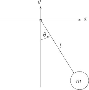
Building systems from parts
The method of using augmented Lagrangians to enforce constraints on dynamical systems provides a way to analyze a compound system by combining the results of the analysis of the parts of the system and the coupling between them.
Consider the compound spring-mass system shown at the top of figure 1.9. We could analyze this as a monolithic system with two configuration coordinates x1 and x2, representing the extensions of the springs from their equilibrium lengths X1 and X2.
An alternative procedure is to break the system into several parts. In our spring-mass system we can choose two parts: one is a spring and mass attached to the wall, and the other is a spring and mass with its attachment point at an additional configuration coordinate ξ. We can formulate a Lagrangian for each part separately. We can then choose a Lagrangian for the composite system as the sum of the two component Lagrangians with a constraint ξ = X1 + x1 to accomplish the coupling.
Let's see how this works. The Lagrangian for the subsystem attached to the wall is
and the Lagrangian for the subsystem that attaches to it is
We construct a Lagrangian for the system composed from these parts as a sum of the Lagrangians for each of the separate parts, with a coupling term to enforce the constraint:
Thus we can write Lagrange's equations for the four configuration coordinates, in order, as follows:
Notice that in this system λ is the force of constraint holding the system together. We can now eliminate the “glue” coordinates ξ and λ to obtain the equations of motion in the coordinates x1 and x2:
This strategy can be generalized. We can make a library of primitive components. Each component may be characterized by a Lagrangian with additional degrees of freedom for the terminals where that component may be attached to others. We then can construct composite Lagrangians by combining components, using constraints to glue together the terminals.
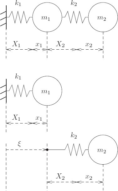
Exercise 1.39: Combining Lagrangians
a. Make another primitive component, compatible with the spring-mass structures described in this section. For example, make a pendulum that can attach to the spring-mass system. Build a combination and derive the equations of motion. Be careful, the algebra is horrible if you choose bad coordinates.
b. For a nice little project, construct a family of compatible mechanical parts, characterized by appropriate Lagrangians, that can be combined in a variety of ways to make interesting mechanisms. Remember that in a good language the result of combining pieces should be a piece of the same kind that can be further combined with other pieces.
Exercise 1.40: Bead on a triaxial surface
Consider again the motion of a bead constrained to move on a triaxial surface (exercise 1.18). Reformulate this using rectangular coordinates as the generalized coordinates with an explicit constraint that the bead must stay on the surface. Find a Lagrangian and show that the Lagrange equations are equivalent to those found in exercise 1.18.
Exercise 1.41: Motion of a tiny golf ball
Consider the motion of a golf ball idealized as a point mass constrained to a frictionless smooth surface of varying height h(x, y) in a uniform gravitational field with acceleration g.
a. Find an augmented Lagrangian for this system, and derive the equations governing the motion of the point mass in x and y.
b. Under what conditions is this approximated by a potential function V (x, y) = mgh(x, y)?
c. Assume that h(x, y) is axisymmetric about x = y = 0. Can you find such an h that yields motions with closed orbits?
1.10.2 Derivative Constraints
Here we investigate velocity-dependent constraints that are “total time derivatives” of velocity-independent constraints. The methods presented so far do not apply because the constraint is velocity-dependent.
Consider a velocity-dependent constraint ψ = 0. That ψ is a total time derivative means that there exists a velocity-independent function φ such that
That φ is velocity-independent means ∂2φ = 0. As state functions the relationship between ψ and φ is
Given a ψ we can find φ by solving this linear partial differential equation. The solution is determined up to a constant, so ψ = 0 implies φ = K for some constant K. On the other hand, if we knew φ = K then ψ = 0 follows. Thus the velocity-dependent constraint ψ = 0 is equivalent to the velocity-independent constraint φ = K, and we know how to find Lagrange equations for such systems.
If L is a Lagrangian for the unconstrained problem, the Lagrange equations with the constraint φ = K are
where λ is a function of time that will be eliminated during the solution process. The constant K does not affect the Lagrange equations. The function φ is independent of velocity, ∂2φ = 0, so the Lagrange equations become
From equation (1.214) we see that
so the Lagrange equations with the constraint ψ = 0 are
The important feature is that we can write the Lagrange equations directly in terms of ψ without having to produce φ. But the validity of these Lagrange equations depends on the existence of φ.
It turns out that the augmented Lagrangian trick also works here. These Lagrange equations are given if we augment the Lagrangian with the constraint ψ multiplied by a function of time λ′:
The Lagrange equations for L′ turn out to be
which, with the identification λ = −Dλ′, are the same as Lagrange equations (1.218).
Sometimes a problem can be naturally formulated in terms of velocity-dependent constraints. The formalism we have developed will handle any velocity-dependent constraint that can be written in terms of the derivative of a coordinate constraint. Such a constraint is called an integrable constraint. Any system for which the constraints can be put in the form of a coordinate constraint, or are already in that form, is called a holonomic system.
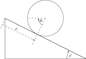
Exercise 1.42: Augmented Lagrangian
Show that the augmented Lagrangian (1.219) does lead to the Lagrange equations (1.220), taking into account the fact that ψ is a total time derivative of φ.
Goldstein's hoop
Here we consider a problem for which the constraint can be represented as a time derivative of a coordinate constraint: a hoop of mass M and radius R rolling, without slipping, down a (one-dimensional) inclined plane (see figure 1.10).96
We will formulate this problem in terms of the two coordinates θ, the rotation of an arbitrary point on the hoop from an arbitrary reference direction, and x, the linear progress down the inclined plane. The constraint is that the hoop does not slip. Thus a change in θ is exactly reflected in a change in x; the constraint function is
This constraint is phrased as a relation among generalized velocities, but it could be integrated to get x = Rθ + c. We may form our augmented Lagrangian with either the integrated constraint or its derivative.
The kinetic energy has two parts, the energy of rotation of the hoop and the energy of the motion of its center of mass.97 The potential energy of the hoop decreases as the height decreases. Thus we may write the augmented Lagrangian:
Lagrange's equations are
And by differentiation of the third Lagrange equation we obtain
By combining these equations we can solve for the dynamical quantities of interest. For this case of a rolling hoop the linear acceleration
is just half of what it would have been if the mass had just slid down a frictionless plane without rotating. Note that for this hoop D2x is independent of both M and R. We see from the Lagrange equations that Dλ can be interpreted as the friction force involved in enforcing the constraint. The frictional force of constraint is
and the angular acceleration is
1.10.3 Nonholonomic Systems
Systems with constraints that are not integrable are termed non-holonomic systems. A constraint is not integrable if it cannot be written in terms of an equivalent coordinate constraint. An example of a nonholonomic system is a ball rolling without slipping in a bowl. As the ball rolls it must turn so that its surface does not move relative to the bowl at the point of contact. This looks as if it might establish a relation between the location of the ball in the bowl and the orientation of the ball, but it doesn't. The ball may return to the same place in the bowl with different orientations depending on the intervening path it has taken. As a consequence, the constraints cannot be used to eliminate any coordinates.
What are the equations of motion governing nonholonomic systems? For the restricted set of systems with nonholonomic constraints that are linear in the velocities, it is widely reported98 that the equations of motion are as follows. Let ψ have the form
a state function that is linear in the velocities. We assume ψ is not a total time derivative. If L is a Lagrangian for the unconstrained system, then the equations of motion are asserted to be
With the constraint ψ = 0, the system is completely specified and the evolution of the system is determined. Note that these equations are identical to the Lagrange equations (1.218) for the case that ψ is a total time derivative, but here the derivation of those equations is no longer valid.
An essential step in the derivation of the Lagrange equations for coordinate constraints φ = 0 with ∂2φ = 0 was to note that two conditions must be satisfied:
and
Because
The Lagrange equations for derivative constraints were derived from this.
This derivation does not go through if the constraint function depends on velocity. In this case, for a variation η to be consistent with the velocity-dependent constraint function ψ it must satisfy (see equation 1.185)
We may no longer eliminate η by the same argument, because η is no longer orthogonal to ∂1ψ ∘ Γ[q], and we cannot rewrite the constraint as a coordinate constraint because ψ is, by assumption, not integrable.
The following is the derivation of the nonholonomic equations from Arnold et al. [6], translated into our notation. Define a “virtual velocity” ξ to be any velocity satisfying
The “principle of d'Alembert–Lagrange,” according to Arnold, states that
for any virtual velocity ξ. Because ξ is arbitrary except that it is required to be orthogonal to ∂2ψ ∘ Γ[q] and any such ξ is orthogonal to
which are the nonholonomic equations.
To convert the stationary action equations to the equations of Arnold we must do the following. To get from equation (1.232) to equation (1.237), we must replace η by ξ. However, to get from equation (1.235) to equation (1.236), we must set η = 0 and replace Dη by ξ. All “derivations” of the nonholonomic equations have similar identifications. It comes down to this: the nonholonomic equations do not follow from the action principle. They are something else. Whether they are correct or not depends on whether or not they agree with experiment.
For systems with either coordinate constraints or derivative constraints, we have found that the Lagrange equations can be derived from a Lagrangian that is augmented with the constraint. However, if the constraints are not integrable the Lagrange equations for the augmented Lagrangian are not the same as the non-holonomic system (equations 1.231).99 Let L′ be an augmented Lagrangian with non-integrable constraint ψ:
then the Lagrange equations associated with the coordinates are
The Lagrange equation associated with λ is just the constraint equation
An interesting feature of these equations is that they involve both λ and Dλ. Thus the usual state variables q and Dq, with the constraint, are not sufficient to determine a full set of initial conditions for the derived Lagrange equations; we need to specify an initial value for λ as well.
In general, for any particular physical system, equations (1.231) and (1.240) are not the same, and in fact they have different solutions. It is not apparent that either set of equations accurately models the physical system. The first approach to nonholonomic systems is not justified by extension of the arguments for the holo-nomic case and the other is not fully determined. Perhaps this indicates that the models are inadequate, that more details of how the constraints are maintained need to be specified.
1.11 Summary
To analyze a mechanical system we construct an action function that gives us a way to distinguish realizable motions from other conceivable motions of the system. The action function is constructed so as to be stationary only on paths describing realizable motions, with respect to variations of the path. This is the principle of stationary action. The principle of stationary action is a coordinate-independent specification of the realizable paths. For systems with or without constraints we may choose any system of coordinates that uniquely determines the configuration of the system.
An action is an integral of a function, the Lagrangian, along the path. For many systems an appropriate Lagrangian is the difference of the kinetic energy and the potential energy of the system. The choice of a Lagrangian for a system is not unique.
For any system for which we have a Lagrangian action we can formulate a system of ordinary differential equations, the Lagrange equations, that is satisfied by any realizable path. The method of deriving the Lagrange equations from the Lagrangian is independent of the coordinate system used to formulate the Lagrangian. One freedom we have in formulation is that the addition of a total time derivative to a Lagrangian for a system yields another Lagrangian that has the same Lagrange equations.
The Lagrange equations are a set of ordinary differential equations: there is a finite state that summarizes the history of the system and is sufficient to determine the future. There is an effective procedure for evolving the motion of the system from a state at an instant. For many systems the state is determined by the coordinates and the rate of change of the coordinates at an instant.
If there are continuous symmetries in a physical system there are conserved quantities associated with them. If the system can be formulated in such a way that the symmetries are manifest in missing coordinates in the Lagrangian, then there are conserved momenta conjugate to those coordinates. If the Lagrangian is independent of time then there is a conserved energy.
1.12 Projects
Exercise 1.43: A numerical investigation
Consider a pendulum: a mass m supported on a massless rod of length l in a uniform gravitational field. A Lagrangian for the pendulum is
For the pendulum, the period of the motion depends on the amplitude. We wish to find trajectories of the pendulum with a given frequency. Three methods of doing this present themselves: (1) solution by the principle of least action, (2) numerical integration of Lagrange's equation, and (3) analytic solution (which requires some exposure to elliptic functions). We will carry out all three and compare the solution trajectories.
Consider the parameters m = 1 kg, l = 1 m, g = 9.8 m s−2. The frequency of small-amplitude oscillations is
a. The angle is periodic in time, so a Fourier series representation is appropriate. We can choose the origin of time so that a zero crossing of the angle is at time zero. Since the potential is even in the angle, the angle is an odd function of time. Thus we need only a sine series. Since the angle returns to zero after one-half period, the angle is an odd function of time about the midpoint. Thus only odd terms of the series are present:
The amplitude of the trajectory is
Find approximations to the first few coefficients An by minimizing the action. You will have to write a program similar to the find-path procedure in section 1.4. Watch out: there is more than one trajectory that minimizes the action.
b. Write a program to numerically integrate Lagrange's equations for the trajectories of the pendulum. The trouble with using numerical integration to solve this problem is that we do not know how the frequency of the motion depends on the initial conditions. So we have to guess, and then gradually improve our guess. Define a function
c. Now let's formulate the analytic solution for the frequency as a function of amplitude. The period of the motion is simply
Using the energy, solve for
Exercise 1.44: Double pendulum behavior
Consider the ideal double pendulum shown in figure 1.11.
a. Formulate a Lagrangian to describe the dynamics. Derive the equations of motion in terms of the given angles θ1 and θ2. Put the equations into a form appropriate for numerical integration. Assume the following system parameters:
|
g |
= | 9.8 m s−2 |
|
l1 |
= | 1.0 m |
|
l2 |
= | 0.9 m |
|
m1 |
= | 1.0 kg |
|
m2 |
= | 3.0 kg |
b. Prepare graphs showing the behavior of each angle as a function of time when the system is started with the following initial conditions:
| θ1(0) | = | π/2 rad |
| θ2(0) | = | π rad |
| = | 0 rad s−1 | |
| = | 0 rad s−1 |
Make the graphs extend to 50 seconds.
c. Make a graph of the behavior of the energy of your system as a function of time. The energy should be conserved. How good is the conservation you obtained?
d. Make a new Lagrangian, for two identical uncoupled double pendulums. (Both pendulums should have the same masses and lengths.) Your new Lagrangian should have four degrees of freedom. Give initial conditions for one pendulum to be the same as in the experiment of part b and give initial conditions for the other pendulum with the m2 bob 10−10 m higher than before. The motions of the two pendulums will diverge as time progresses. Plot the logarithm of the absolute value of the difference of the positions of the m2 bobs in your two pendulums against the time. What do you see?
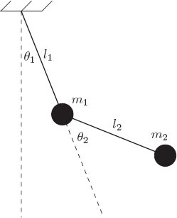
e. Repeat the previous comparison, but this time use the base initial conditions:
| θ1(0) | = | π/2 rad |
| θ2(0) | = | 0 rad |
| = | 0 rad s−1 | |
| = | 0 rad s−1 |
What do you see here?
1A stationary point of a function is a point where the function's value does not vary as the input is varied. Local maxima or minima are stationary points.
2The variational formulation successfully describes all of the Newtonian mechanics of particles and rigid bodies. The variational formulation has also been usefully applied in the description of many other systems such as classical electrodynamics, the dynamics of inviscid fluids, and the design of mechanisms such as four-bar linkages. In addition, modern formulations of quantum mechanics and quantum field theory build on many of the same concepts. However, it appears that not all dynamical systems have a variational formulation. For example, there is no simple prescription to apply the variational apparatus to systems with dissipation, though in special cases variational methods can still be used.
3We often refer to a point particle with mass but no internal structure as a point mass.
4Strictly speaking, the dimension of the configuration space and the number of degrees of freedom are not the same. The number of degrees of freedom is the dimension of the space of configurations that are “locally accessible.” For systems with integrable constraints the two are the same. For systems with non-integrable constraints the configuration dimension can be larger than the number of degrees of freedom. For further explanation see the discussion of systems with non-integrable constraints in section 1.10.3. Apart from that discussion, all of the systems we consider have integrable constraints (they are “holonomic”). This is why we have chosen to blur the distinction between the number of degrees of freedom and the dimension of the configuration space.
5A tuple is an ordered list of elements. An element may itself be a tuple.
6A tuple of functions that all have the same domain is itself a function on that domain: Given a point in the domain, the value of the tuple of functions is a tuple of the values of the component functions at that point.
7The use of superscripts to index the coordinate components is traditional, even though there is potential confusion with exponents. We use zero-based indexing.
8More precisely, the generalized coordinates identify open subsets of the configuration space with open subsets of Rn. It may require more than one set of generalized coordinates to cover the entire configuration space. For example, if the configuration space is a two-dimensional sphere, we could have one set of coordinates that maps (a little more than) the northern hemisphere to a disk, and another set that maps (a little more than) the southern hemisphere to a disk, with a strip near the equator common to both coordinate systems. A space that can be locally parameterized by smooth coordinate functions is called a differentiable manifold.
9Here ∘ denotes composition of functions: (f ∘ g)(t) = f(g(t)).
10The derivative of a function f is a function, denoted Df. Our notational convention is that D is a high-precedence operator. Thus D operates on the adjacent function before any other application occurs: Df(x) is the same as (Df)(x).
11Experience with systems on an atomic scale suggests that at this scale systems do not travel along well-defined configuration paths. To describe the evolution of systems on the atomic scale we employ quantum mechanics. Here, we restrict attention to systems for which the motion is well described by a smooth configuration path.
12Extrapolation of the orbit of the Moon backward in time cannot determine the point at which it was placed on this trajectory. To determine the origin of the Moon we must supplement dynamical evidence with other physical evidence such as chemical compositions.
13We suspect that this argument can be promoted to a precise constraint on the possible ways of making this path-distinguishing function.
14Historically, Huygens was the first to use the term “action” in mechanics, referring to “the effect of a motion.” This is an idea that came from the Greeks. In his manuscript “Dynamica” (1690) Leibniz enunciated a “Least Action Principle” using the “harmless action,” which was the product of mass, velocity, and the distance of the motion. Leibniz also spoke of a “violent action” in the case where things collided.
15A definite integral of a real-valued function f of a real argument is written
16Traditionally, square brackets are put around functional arguments. In this case, the square brackets remind us that the value of S may depend on the function q in complicated ways, such as through its derivatives.
17In the case of a real-valued function, the value of the function and its derivatives at some point can be used to construct a power series. For sufficiently nice functions (real analytic), the power series constructed in this way converges in some interval containing the point. Not all functions can be locally represented in this way. For example, the function f(x) = exp(−1/x2), with f(0) = 0, is zero and has all derivatives zero at x = 0, but this infinite number of derivatives is insufficient to determine the function value at any other point.
18In our notation the application of a path-dependent function to its path is of higher precedence than the composition, so L ∘ Γ[q] = L ∘ (Γ[q]).
19We will later discover that an initial segment of the local tuple is sufficient to determine the future evolution of the system. That a configuration and a finite number of derivatives determine the future means that there is a way of determining all of the rest of the derivatives of the path from the initial segment.
20The classical Lagrangian plays a fundamental role in the path-integral formulation of quantum mechanics (due to Dirac and Feynman), where the complex exponential of the classical action yields the relative probability amplitude for a path. The Lagrangian is the starting point for the Hamiltonian formulation of mechanics (discussed in chapter 3), which is also essential in the Schrödinger and Heisenberg formulations of quantum mechanics and in the Boltzmann–Gibbs approach to statistical mechanics.
21The principle becomes the “principle of least action” if the path is sufficiently short. In the more general case the action is stationary. The term “principle of least action” is also commonly used to refer to a result, due to Maupertuis, Euler, and Lagrange, which says that free particles move along paths for which the integral of the kinetic energy is minimized among all paths with the given endpoints. Correspondingly, the term “action” is sometimes used to refer specifically to the integral of the kinetic energy. (Actually, Euler and Lagrange used the vis viva, or twice the kinetic energy.)
22Other ways of stating the principle of stationary action make it sound teleological and mysterious. For instance, one could imagine that the system considers all possible paths from its initial configuration to its final configuration and then chooses the one with the smallest action. Indeed, the underlying vision of a purposeful, economical, and rational universe played no small part in the philosophical considerations that accompanied the initial development of mechanics. The earliest action principle that remains part of modern physics is Fermat's principle, which states that the path traveled by a light ray between two points is the path that takes the least amount of time. Fermat formulated this principle around 1660 and used it to derive the laws of reflection and refraction. Motivated by this, the French mathematician and astronomer Pierre-Louis Moreau de Maupertuis enunciated the principle of least action as a grand unifying principle in physics. In his Essai de cosmologie (1750) Maupertuis appealed to this principle of “economy in nature” as evidence of the existence of God, asserting that it demonstrated “God's intention to regulate physical phenomena by a general principle of the highest perfection.” For a historical perspective on Maupertuis's, Euler's, and Lagrange's roles in the formulation of the principle of least action, see [28].
23For reflection the angle of incidence is equal to the angle of reflection. Refraction is described by Snell's law: when light passes from one medium to another, the ratio of the sines of the angles made to the normal to the interface is the inverse of the ratio of the refractive indices of the media. The refractive index is the ratio of the speed of light in the vacuum to the speed of light in the medium.
24Here we are making a function definition. A definition specifies the value of the function for arbitrarily chosen formal parameters. One may change the name of a formal parameter, so long as the new name does not conflict with any other symbol in the definition. For example, the following definition specifies exactly the same free-particle Lagrangian:
25The Lagrangian is formally a function of the local tuple, but any particular Lagrangian depends only on a finite initial segment of the local tuple. We define functions of local tuples by explicitly declaring names for the elements of the initial segment of the local tuple that includes the elements upon which the function depends.
26 We represent the local tuple as a composite data structure, the components of which are the time, the generalized coordinates, the generalized velocities, and possibly higher derivatives. We do not want to be bothered by the details of packing and unpacking the components into these structures, so we provide utilities for doing this.
27Be careful. The x in the definition of q is not the same as the x that was used as a formal parameter in the definition of the free-particle Lagrangian above. There are only so many letters in the alphabet, so we are forced to reuse them. We will be careful to indicate where symbols are given new meanings.
28A tuple of coordinate or velocity components is made with the procedure up. Component i of the tuple q is (ref q i). All indexing is zero based. The word up is to remind us that in mathematical notation these components are indexed by superscripts. There are also down tuples of components that are indexed by subscripts. See the appendix on notation.
The constructor up is also used to package the time, the coordinates, and the velocities into a data structure representing a local tuple. The selectors time, coordinate, and velocity extract the appropriate pieces from the local structure. The procedure time is the same as the procedure (component 0), and similarly coordinate is (component 1) and velocity is (component 2).
29Derivatives of functions yield functions. For example, ((D cube) 2) => 12 and ((D cube) 'a) => (* 3 (expt a 2)).
30Although Γ produces an arbitrarily long local tuple, our procedure Gamma produces by default only the first three elements. If a longer local tuple is needed, Gamma can be given the length of the required tuple as an extra argument.
31In our system, arithmetic operators are generic over symbolic expressions as well as numeric values; arithmetic procedures can work uniformly with numbers or expressions. For example, given the procedure (define (cube x) (* x x x)) we can obtain its value for a number (cube 2) => 8 or for a literal symbol (cube 'a) => (* a a a).
32For very complicated expressions the prefix notation of Scheme is often better, but simplification is almost always useful. We can separate the functions of simplification and infix display. We will see examples of this later.
33Scmutils includes a variety of numerical integration procedures. The examples in this section were computed by rational-function extrapolation of Euler–MacLaurin formulas with a relative error tolerance of 10−10.
34For a real physical situation we would have to specify units for these quantities, but in this illustration we leave them unspecified.
35Here we use numerals with decimal points to specify the parameters. This forces the representations to be floating point, which is efficient for numerical calculation. If symbolic algebra is to be done it is essential that the numbers be exact integers or rational fractions, so that expressions can be reliably reduced to lowest terms. Such numbers are specified without a decimal point.
36The squared magnitude of the velocity is
37Note that we are doing arithmetic on functions. We extend the arithmetic operations so that the combination of two functions of the same type (same domains and ranges) is the function on the same domain that combines the values of the argument functions in the range. For example, if f and g are functions of t, then fg is the function t ↦ f(t)g(t). A constant multiple of a function is the function whose value is the constant times the value of the function for each argument: cf is the function t ↦ cf(t).
38Note that we are adding procedures. Paralleling our extension of arithmetic operations to functions, arithmetic operations are extended to compatible procedures.
39The arguments to minimize are a procedure implementing the univariate function in question, and the lower and upper bounds of the region to be searched. Scmutils includes a choice of methods for numerical minimization; the one used here is Brent's algorithm, with an error tolerance of 10−5. The value returned by minimize is a list of three numbers: the first is the argument at which the minimum occurred, the second is the minimum obtained, and the third is the number of iterations of the minimization algorithm required to obtain the minimum.
40Yes, -1.5987211554602254e-14 is zero for the tolerance required of the minimizer. And 435.0000000000237 is arguably the same as 435 obtained before.
41There are lots of good ways to make such a parametric set of approximating trajectories. One could use splines or higher-order interpolating polynomials; one could use Chebyshev polynomials; one could use Fourier components. The choice depends upon the kinds of trajectories one wants to approximate.
42Here is one way to implement make-path:
(define (make-path t0 q0 t1 q1 qs)
  (let ((n (length qs)))
    (let ((ts (linear-interpolants t0 t1 n)))
      (Lagrange-interpolation-function
        (append (list q0) qs (list q1))
        (append (list t0) ts (list t1))))))
The procedure linear-interpolants produces a list of elements that linearly interpolate the first two arguments. We use this procedure here to specify ts, the n evenly spaced intermediate times between t0 and t1 at which the path will be specified. The parameters being adjusted, qs, are the positions at these intermediate times. The procedure Lagrange-interpolation-function takes a list of values and a list of times and produces a procedure that computes the Lagrange interpolation polynomial that passes through these points.
43The minimizer used here is the Nelder–Mead downhill simplex method. As usual with numerical procedures, the interface to the nelder-mead procedure is complex, with lots of optional parameters to let the user control errors effectively. For this presentation we have specialized nelder-mead by wrapping it in the more palatable multidimensional-minimize. Unfortunately, you will have to learn to live with complicated numerical procedures someday.
44Don't worry. We know that you don't yet know why this is the right Lagrangian. We will get to this in section 1.6.
45The square of a structure of components is defined to be the sum of the squares of the individual components.
46By convention, named constants have names that begin with a colon. The constants named :pi and :-pi are what we would expect from their names.
47The derivative or partial derivative of a function that takes structured arguments is a new function that takes the same number and type of arguments. The range of this new function is itself a structure with the same number of components as the argument with respect to which the function is differentiated. See the appendix on notation for more.
48To make this argument more precise requires careful analysis.
49The variation operator δη is like the derivative operator in that it acts on the immediately following function: δηf[q] = (δηf)[q].
50We separate out the definition of g: We cannot substitute Dq for g[q] in δηg[q] because δη applies to g not g[q].
51The type of a literal function is described by a function signature. The default function signature is (-> Real Real) indicating a real-valued function of a real argument. In this case F is declared as a function that is shaped like a Lagrangian, with an unspecified number of degrees of freedom. For more information about function signatures see the appendix on notation.
52A function of multiple arguments is considered a function of an up tuple of its arguments. Thus, the derivative of a function of multiple arguments is a down tuple of the partial derivatives of that function with respect to each of the arguments. So in the case of a Lagrangian L,
53When we write a definition that names the components of the local tuple, we indicate that these are grouped into time, position, and velocity components by separating the groups with semicolons.
54The symbol
55In traditional notation these equations read
56The Lagrange-equations procedure uses the operations (partial 1) and (partial 2), which implement the partial derivative operators with respect to the second and third argument positions (those with indices 1 and 2).
57There is a Lagrange equation for every degree of freedom. The residuals of all the equations are zero if the path is realizable. The residuals are arranged in a down tuple because they result from derivatives of the Lagrangian with respect to argument slots that take up tuples. See the appendix on notation.
58Observe that the second derivative is indicated as the square of the derivative operator (expt D 2). Arithmetic operations in Scmutils extend over operators as well as functions.
59Remember that x and v are just formal parameters of the Lagrangian. This x is not the path x used earlier in the derivation, though it could be the value of that path at a particular time.
60We can always give a function extra arguments that are not used so that it can be algebraically combined with other functions of the same shape.
61William Rowan Hamilton formulated the fundamental variational principle for time-independent systems in 1834–1835. Jacobi gave this principle the name “Hamilton's principle.” For systems subject to generic, nonstationary constraints Hamilton's principle was investigated in 1848 by Ostrogradsky, and in the Russian literature Hamilton's principle is often called the Hamilton–Ostrogradsky principle.
Hamilton (1805–1865) was a brilliant mathematician. His early work on geometric optics (based on Fermat's principle) was so impressive that he was elected to the post of Professor of Astronomy at Trinity College and Royal Astronomer of Ireland while he was still an undergraduate. He produced two monumental works of mathematics. His discovery of quaternions revitalized abstract algebra and sparked the development of vector techniques in physics. His 1835 memoir “On a General Method in Dynamics” put variational mechanics on a firm footing, finally giving substance to Maupertuis's vaguely stated Principle of Least Action of 100 years before. Hamilton also wrote poetry and carried on an extensive correspondence with Wordsworth, who advised him to put his energy into writing mathematics rather than poetry.
In addition to the formulation of the fundamental variational principle, Hamilton also emphasized the analogy between geometric optics and mechanics, and stressed the importance of the momentum variables (which were earlier introduced by Lagrange and Cauchy), leading to the “canonical” form of mechanics discussed in chapter 3.
62When applied to a tuple, square means the sum of the squares of the components of the tuple.
63As described in footnote 26 above, the procedure up constructs a local tuple from an initial segment of time, coordinates, and velocities.
64We hope you appreciate the TEX magic here. Symbols with carets, underlines, the names of Greek letters, and those terminating in the characters “dot” are converted by show-expression to the corresponding TEX expression.
65We will simply accept the Newtonian procedure for systems with rigid constraints and find Lagrangians that are equivalent. Of course, actual bodies are never truly rigid, so we may wonder what detailed approximations have to be made to treat them as if they were truly rigid. For instance, a more satisfying approach would be to replace the rigid distance constraints by very stiff springs. We could then immediately write the Lagrangian as L = T − V, and we should be able to derive the Newtonian procedure for systems with rigid constraints as an approximation. However, this is too complicated to do at this stage, so we accept the Newtonian idealization.
66This Lagrangian is purely formal and does not represent a model of the constraint forces. In particular, note that the constraint terms do not add up to a potential energy with a minimum when the constraints are exactly satisfied. Rather, the constraint terms in the Lagrangian are zero when the constraint is satisfied, and can be either positive or negative depending on whether the distance between the particles is larger or smaller than the constraint distance.
67Typically the number of components of x is equal to the sum of the number of components of q and c; adding a strut removes a degree of freedom and adds a distance constraint. However, there are singular cases in which the addition of single strut can remove more than a single degree of freedom. We do not consider the singular cases here.
68Consider a function g of, say, three arguments, and let g0 be a function of two arguments satisfying g0(x, y) = g(x, y, 0). Then (∂0g0)(x, y) = (∂0g)(x, y, 0). The substitution of a value in an argument commutes with the taking of the partial derivative with respect to a different argument. In deriving the Lagrange equations for q we can set c = l and
69Rz(α) yields a function that rotates its argument about the ẑ axis by the angle α, and Ry is similar.
70Components of a tuple structure, such as the value of Γ[q](t), can be selected with selector functions: Ii gets the element with index i from the tuple.
71The Lipschitz condition is that the rate of change of the state is bounded by a constant in an open set around each state. See [25] for a good treatment of the Lipschitz condition.
72If the coordinates are redundant we cannot, in general, solve for the highest-order derivative. However, since we can transform to irredundant coordinates, since we can solve the initial-value problem in the irredundant coordinates, and since we can construct the redundant coordinates from the irredundant coordinates, we can in general solve the initial-value problem for redundant coordinates. The only hitch is that we cannot specify arbitrary initial conditions: the initial conditions must be consistent with the constraints.
73We may encounter singularities that make this matrix uninvertable, but in real systems these singularities are isolated and can be avoided by changing coordinates.
74For Lagrangians that depend on time, coordinates, and velocities the state is specified by time, coordinates, and velocities. However, if a Lagrangian depends on the first four components of the local tuple (time, coordinates, velocities, and accelerations) the state of the system will be specified by the first five components of the local tuple.
75The procedure solve-linear-left multiplies its second argument by the inverse of its first argument on the left. So, if u = Mv then v = M−1u; (solve-linear-left M u) produces v.
76The Scmutils system provides a variety of numerical integration routines that can be accessed through this interface. These include quality-controlled Runge–Kutta and Bulirsch–Stoer. The default integration method is Bulirsch–Stoer.
77The procedure state-advancer automatically compiles state-derivative procedures the first time they are encountered. The first time a new state derivative is used there is a delay while compilation occurs.
78The results are plotted in a plot window created by the procedure frame with arguments xmin, xmax, ymin, and ymax that specify the limits of the plotting area. Points are added to the plot with the procedure plot-point that takes a plot window and the abscissa and ordinate of the point to be plotted.
The procedure principal-value is used to reduce an angle to a standard interval. The argument to principal-value is the point at which the circle is to be cut. Thus (principal-value :pi) is a procedure that reduces an angle θ to the interval −π ≤ θ < π.
79In older literature conserved quantities are sometimes called first integrals.
80Observe that we indicate a component of the generalized momentum with a subscript, and a component of the generalized coordinates with a superscript. These conventions are consistent with those commonly used in tensor algebra, which is sometimes helpful in working out complex problems.
81For example, we may construct equivalent Lagrangians that differ only by a total time derivative. The momentum state functions for these Lagrangians are different.
82In general, conserved quantities in a physical system are associated with continuous symmetries, whether or not one can find a coordinate system in which the symmetry is apparent. This powerful notion was formalized and a theorem linking conservation laws with symmetries was proved by Noether early in the 20th century. See section 1.8.5 on Noether's theorem.
83The sign of the energy state function is a matter of convention.
84We may construct equivalent Lagrangians that differ only by a total time derivative. The energy state functions for these Lagrangians are different.
85A function f is homogenous of degree n if and only if f(ax) = anf(x). Euler's theorem says that if f is a homogeneous function of degree n, then Df(x)x = nf(x). The proof is as follows: Let gx(a) = f(ax). Then Dgx(a) = Df(ax)x. But gx(a) = anf(x) by the definition of homogeneity. Therefore Dgx(a) = nan−1f(x). Equating these, we find Df(ax)x = nan−1f(x). Specializing to a = 1 we obtain Df(x)x = nf(x) as required.
86Traditionally the Jacobi constant is defined as CJ = −2ℰ.
87The total time derivative is like a derivative with respect to a real-number argument in that it does not generate structure, so it can commute with derivatives that generate structure. Be careful, though: it may not commute with some derivatives for other reasons. For example,
88The definition of the procedure Rx is
(define ((Rx angle) q)
  (let ((ca (cos angle)) (sa (sin angle)))
    (let ((x (ref q 0)) (y (ref q 1)) (z (ref q 2)))
      (up x
          (- (* ca y) (* sa z))
          (+ (* sa y) (* ca z))))))
The definitions of Ry and Rz are similar. See footnote 69.
89The local-tuple function f is the same as the local-tuple function
90This F->C is more general than the code introduced on page 46 in that it allows computation of transformations of higher derivatives of the local tuple, if required.
To make this work, Gamma is also extended to generate more elements of the local tuple than are needed for Lagrangians that depend on time, coordinates, and velocities. Here Gamma is given one more argument than it usually has. This optional argument gives the length of the initial segment of the local tuple needed. The default length is 3, giving components of the local tuple up to and including the velocities.
91Given any acceptable variation, we may make another acceptable variation by multiplying the given one by a bump function that emphasizes any particular time interval.
92We take two tuple-valued functions of time to be orthogonal if at each instant the dot product of the tuples is zero. Similarly, tuple-valued functions are considered parallel if at each moment one of the tuples is a scalar multiple of the other. The scalar multiplier is in general a function of time.
93Recall that the Euler–Lagrange operator
94This constraint has the same form as those used in the demonstration that L = T − V can be used for rigid systems. Here it is a particular example of a more general set of constraints.
95Indeed, if we had scaled the constraint equations as we did in the discussion of Newtonian constraint forces, we could have identified λ with the the magnitude of the constraint force F. However, though λ will in general be related to the constraint forces it will not be one of them. We chose to leave the scaling as it naturally appeared rather than make things turn out artificially pretty.
96This example appears in [20], pp. 49–51,
97We will see in chapter 2 how to compute the kinetic energy of rotation, but for now the answer is
98For some treatments of nonholonomic systems see, for example, Whittaker [46], Goldstein [20], Gantmakher [19], or Arnold et al. [6].
99Arnold et al. [6] call the variational mechanics with the constraints added to the Lagrangian Vakonomic mechanics.