Tutorial: Basic Analysis

This tutorial is designed to briefly walk new EpiInf users through the process of inferring epidemiological parameters and prevalence trajectories from a set of serially-sampled genetic sequence data.

Loading an alignment

For this tutorial, we will use a set of simulated sequence data which is included with the EpiInf package. To load this aligment, open BEAUti and set the working directory to the EpiInf package directory by opening the “File” menu, finding the “Set working dir” submenu and selecting “EpiInf”:

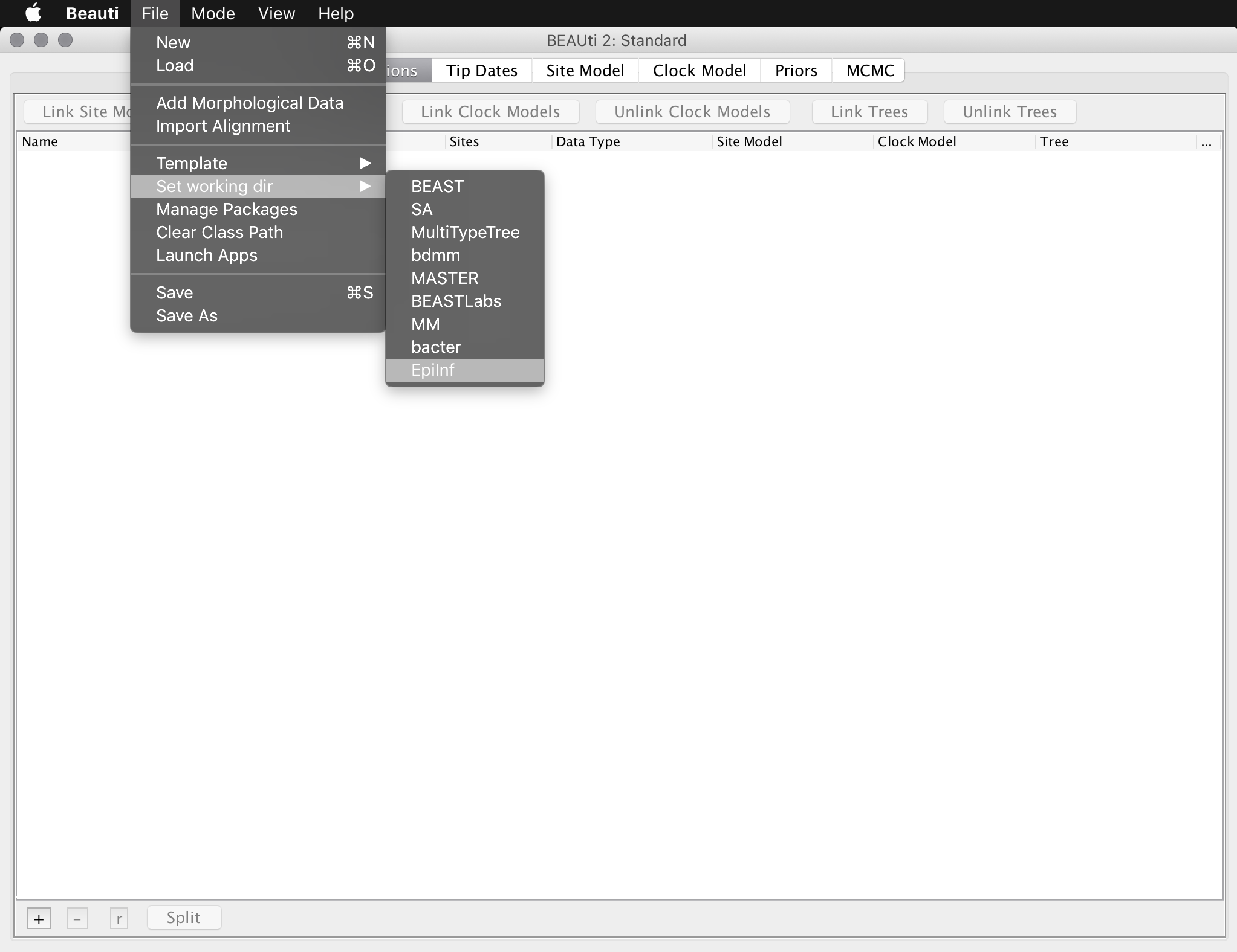
Be aware that the previous step is only required for this tutorial: it is just included to make it easier to locate the example data. It is not required when loading your own data.

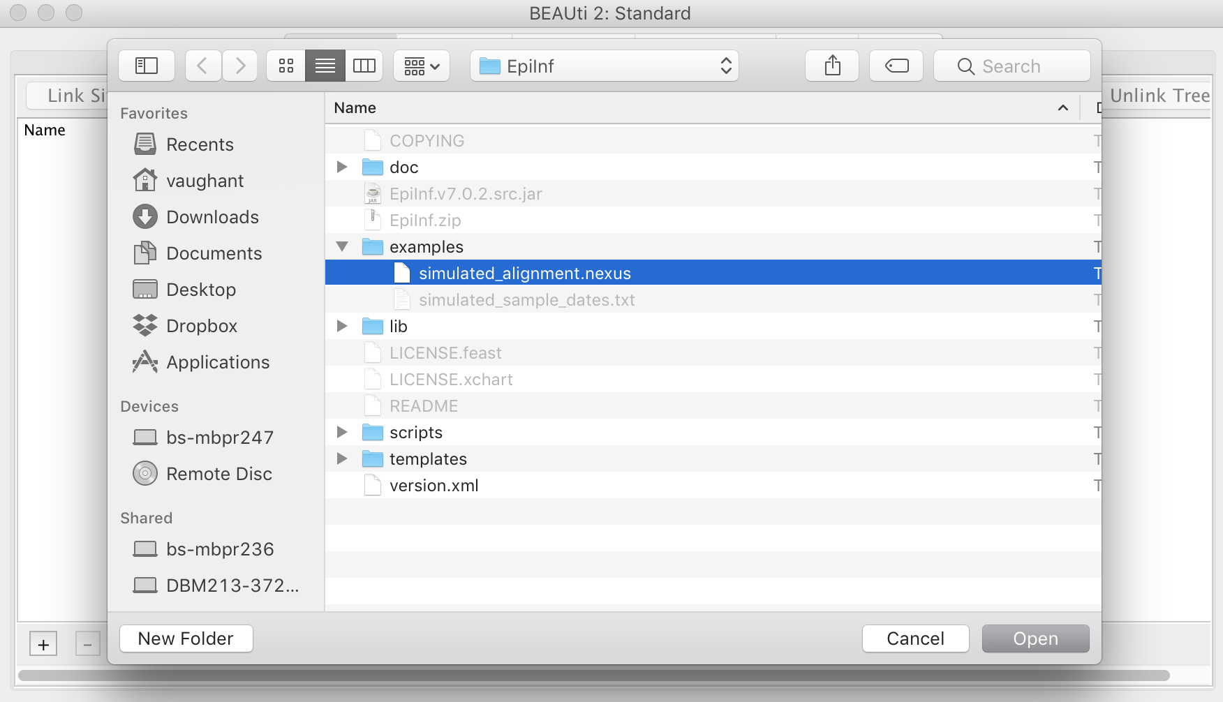
Now import the simulated sequence alignment into BEAUti, which is named “simulated_alignment.nexus”:

Setting up site model, tip dates and clock model

This sequence data were sampled over the entire period of the epidemic. The simulated sample times are provided in a separate file named “simulated_sample_ages.txt”. This file contains a tab-delimited table where each row contains a taxon (sequence) name and its associated age with respect to the most recent sample:

t0	0.0
t1	0.02713882328
t2	0.497098185552
t3	0.789029282226
t4	0.804044538371
t5	1.01584369467
t6	1.20734565128
t7	1.28156508475
t8	1.35845381067
t9	1.35850615159
...

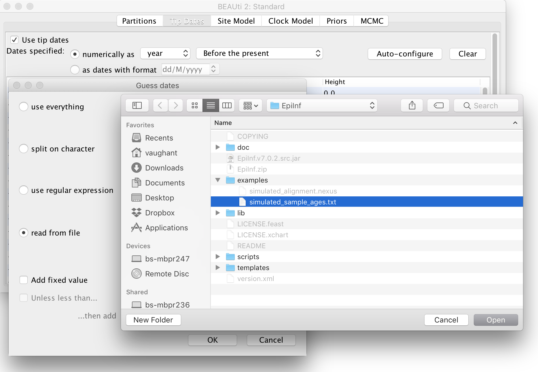
To assign these times to the sequences, open the “Tip Dates” panel and select the check box “Use tip dates”. (Otherwise BEAUti will assume all sequences were sampled at a single time.) Then, set the dates to be specified numerically as years before the present by selecting “before the present” from the combo-box. Finally, press the “Auto-configure” button, select “read from file” and choose the file “simulated_sample_ages.txt”:

The site (substitution) model we will use is the basic Jukes-Cantor model. Open the “Site Model” panel in BEAUti and ensure that this is selected. (It is the default.) Be aware that this model should generally not be used for real data: we are using it here only because our data are artificial.

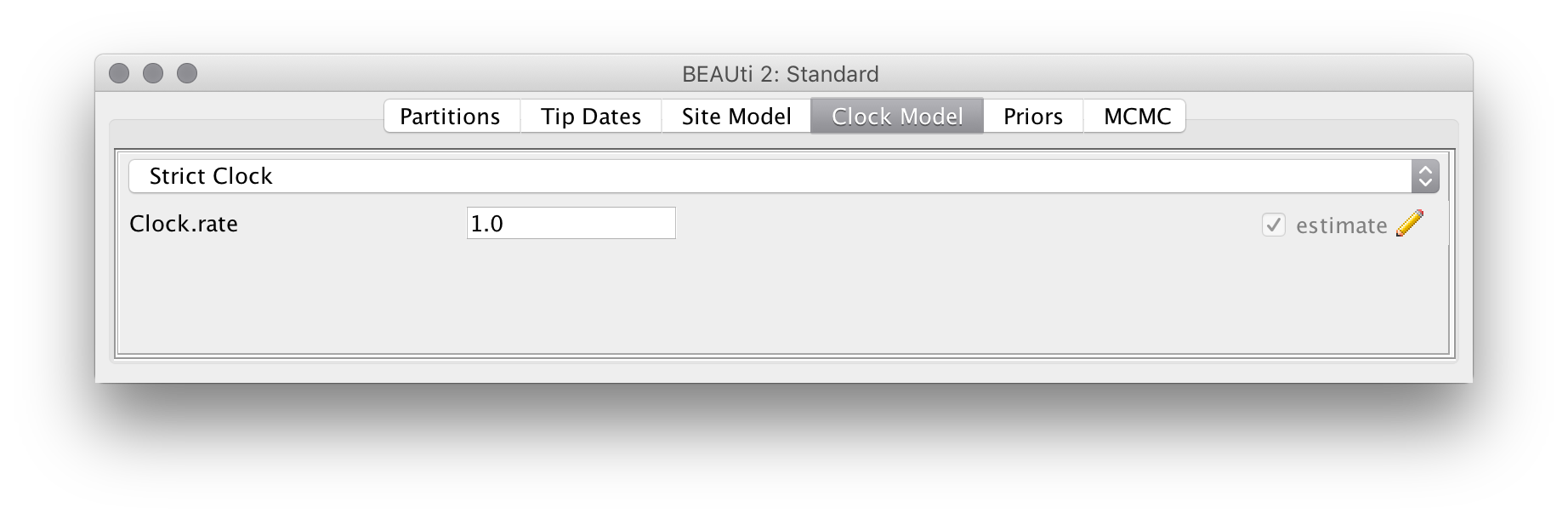
Similarly, we will use a strict clock model for this analysis. Since we have samples taken through time the clock rate becomes identifiable and will thus be estimated by default. To speed up the analysis we will change the starting value of this rate to 0.01, which is closer to the true value:

Setting up the EpiInf tree prior

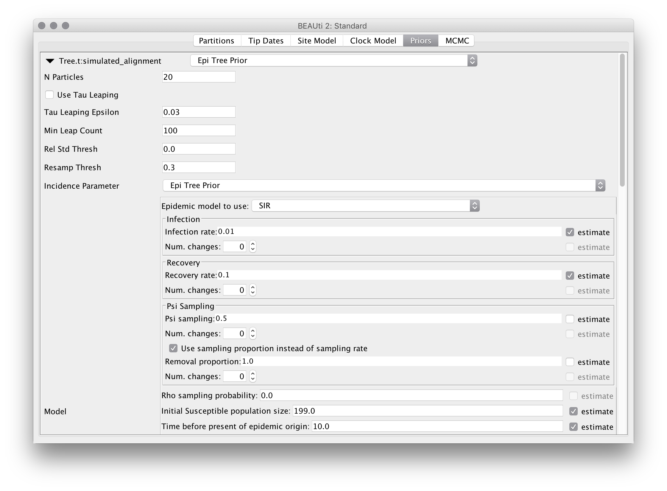
The core of EpiInf is a particle filter based algorithm for computing transmission tree densities conditional on parameters of epidemiological models. Switch to the “Priors” panel in BEAUti andselect “Epi Tree Prior” as the tree prior. Then, expand the options for this prior by clicking the arrow immediately to the left.

For this analysis we will use just 20 particles per tree prior evaluation instead of the default 100. Reducing this number increases the noise in the particle filter estimate of the tree prior density, but improves the speed of the analysis. However, be aware that there is a trade-off: the increased noise can lead to slower mixing overall.

Select the “SIR model” from the list of epidemic models and select the option to “use sampling proportion instead of sampling rate”. This causes the “psi sampling variable” to represent the sampling proportion (psi/(psi+mu)) rather than the absolute rate of the linear psi-sampling process. Deselect the “estimate” button to the right of the parameter. The top portion of the prior panel should now appear as below:

Be aware that although we don’t use this feature here, each of the sampling rate, infection rate and recovery rate parameters may vary be given the ability to vary in a piecewise-constant manner through time. To allow for piecewise-constant variation, simply increase the “Num. changes” values from 0 and specify the times at which the changes should occur (as ages relative to the end of the sampling period). These ages can also be estimated by selecting the checkbox that appears to their right.

Once the model and the intial parameter values are defined, the figure at the bottom of the panel is updated to show a number of prevalence trajectories simulated under that model. For our configuration, you should see something like the following:

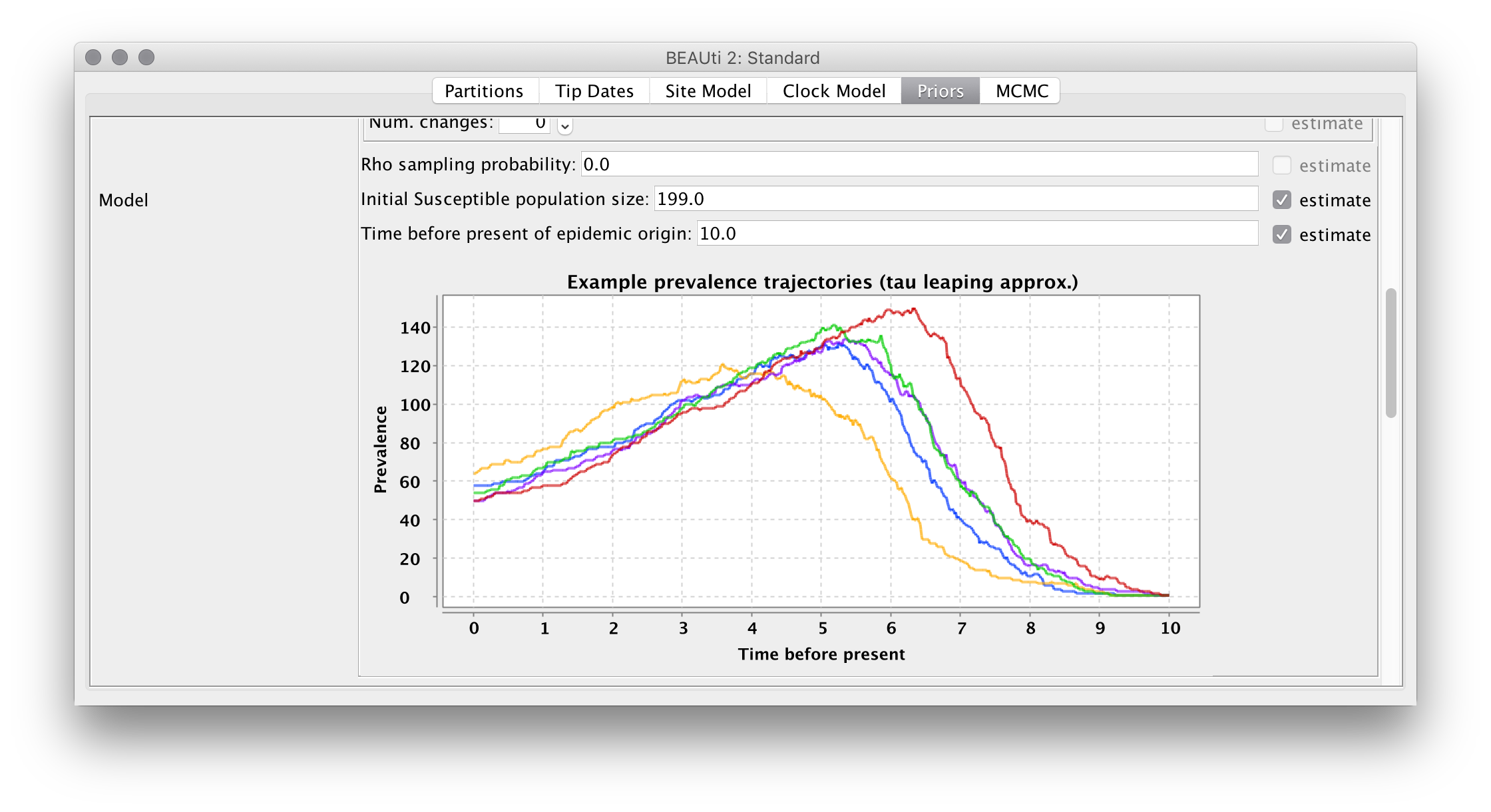
Note that the variation between the example trajectories is purely due to the noise in the demographic process.

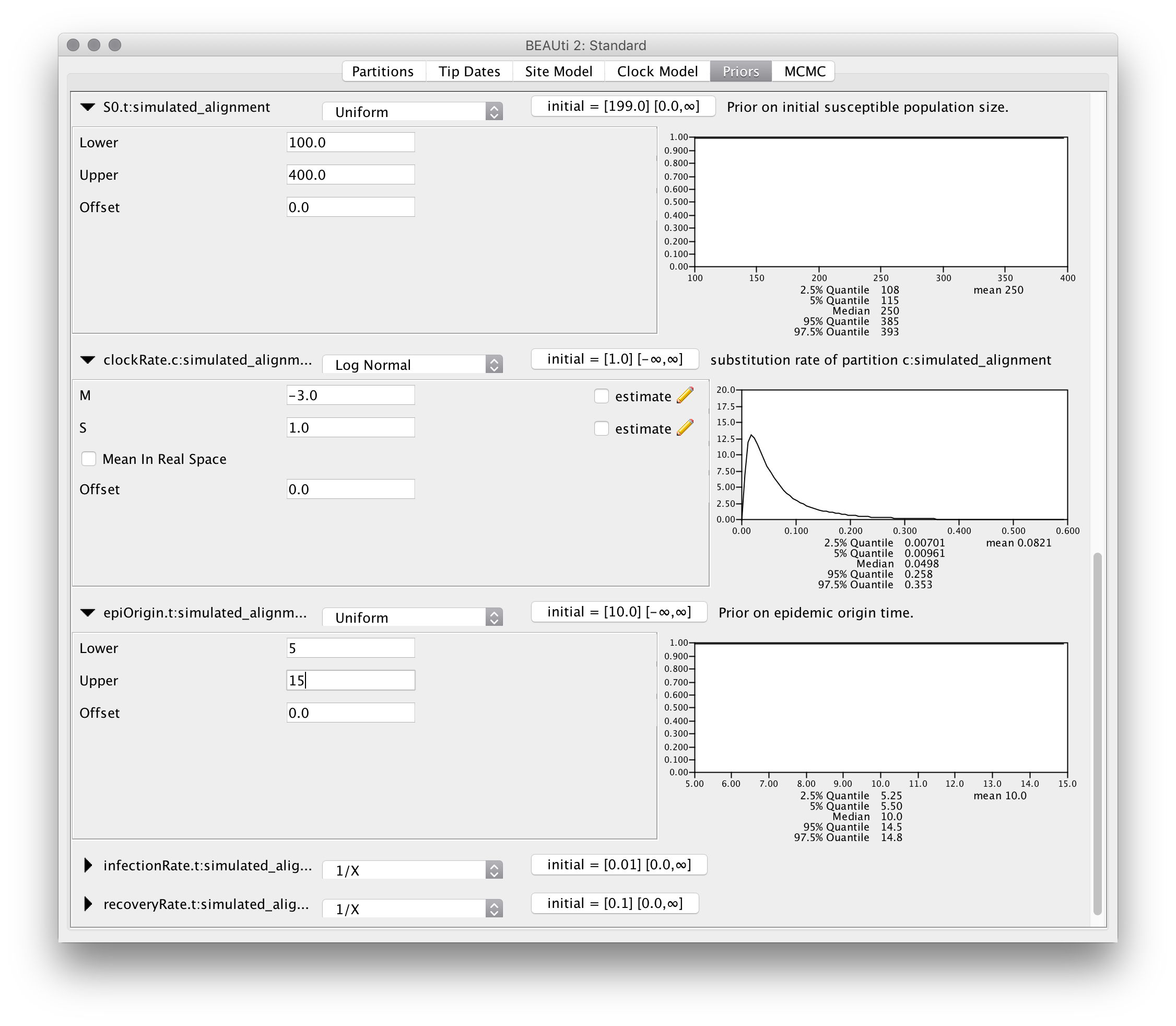
Parameter priors

Finally, set the parameter priors as follows:

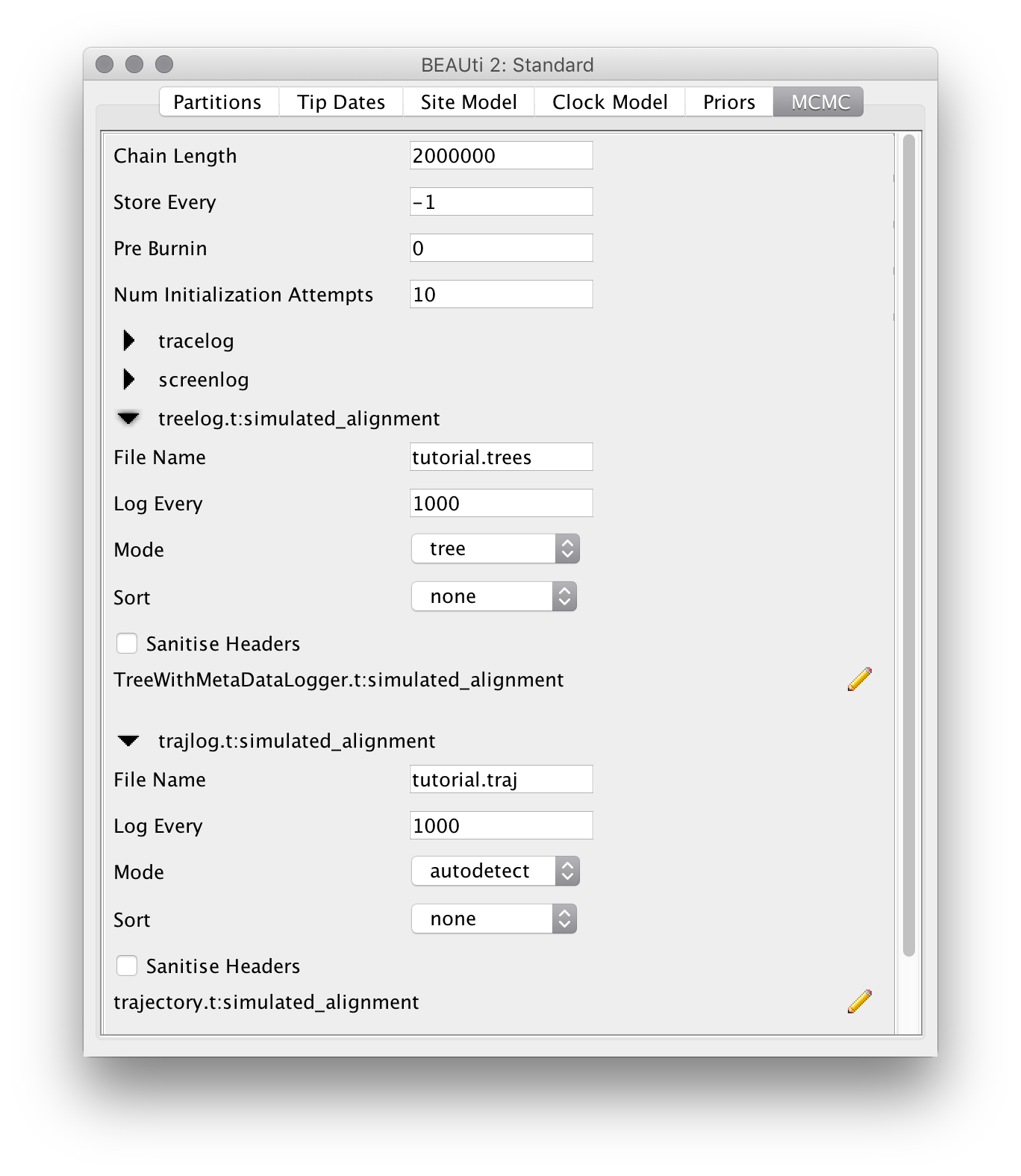
MCMC options

For this exampel analysis we will use a short chain of 2 million iterations. To make things neater, we also change the output filenames for the trace, tree and trajectory logs to tutorial.log, tutorial.trees and tutorial.traj, respectively:

Running the analysis

Run the analysis just as you would any other BEAST 2 analysis. That is,

1. Start BEAST 2.
2. Select the XML you produced in the previous section from the file selection dialog box.

Once BEAST is running, you should see output periodically printed to standard out (if you’re running BEAST from a terminal emulator) or the output window. The analysis we’ve set up should take around half an hour to complete on a modern computer.

Analyzing the results

During the analysis results are written to several files which can usually located in the same directory as the directory containing the input XML. These are:

1. The log file, which ends in the extension .log and contains sampled parameter values,
2. The tree file, which ends in the extension .trees and contains sampled trees.
3. The traj file, which ends in the extension .traj and contains sampled stochastic population trajectories.

Parameter posteriors

As usual, we can examine the posteriors for the model parameters by loading the trace log file (here tutorial.log) into the programme Tracer:

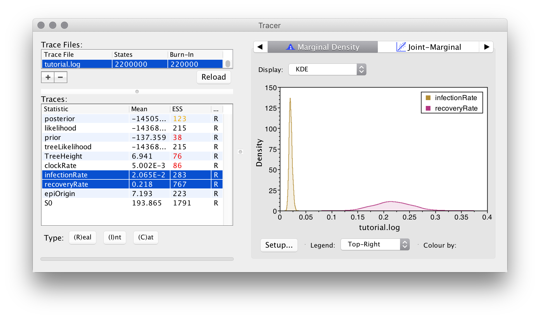
Apart from the usual ESS values, something to pay close attention to in EpiInf analyses is the trace for the tree height:

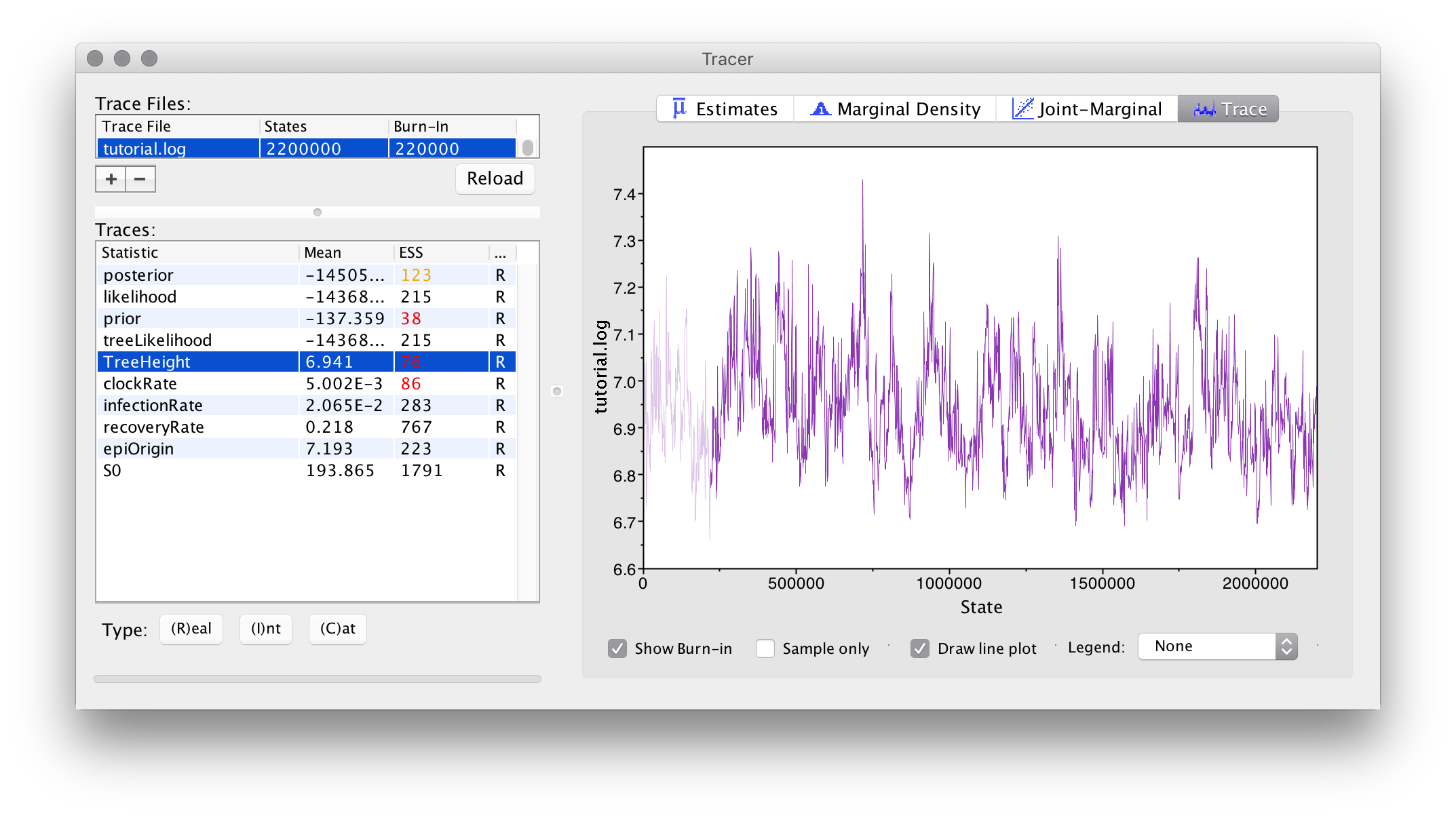
If this trace contains large numbers of iterations where the sampled value remained completely unchanged (became “stuck”), we are likely using too few particles to compute the tree prior estimate, as noisy estimates (which still being correct in the limit of an infinitely long chain) produce this behaviour if the amplitude of the noise is too large.

Happily, we haven’t observed this behaviour in our example analysis: although you may wish to repeat the analysis with an even smaller number of particles and compare the result.

Tree posteriors

In this analysis we are largely uninterested in the sampled trees, but of course they can be summarized and visualized in the same way as for other BEAST 2 analyses.

Trajectory posteriors

In order to visualize the trajectory posterior, we can use an R script which is distributed with the EpiInf package. To load this script, start R and set the working directory (either using the setwd() or using the appropriate menu option in your favourite R GUI) to the directory containing your analysis output files.

Then, open the package manager in BEAUti (File->Manage packages) and press the button marked “?” in the lower-right corner. This should bring up a message dialog explaining where to find installed BEAST 2 packages. For instance, this is what appears on my system:

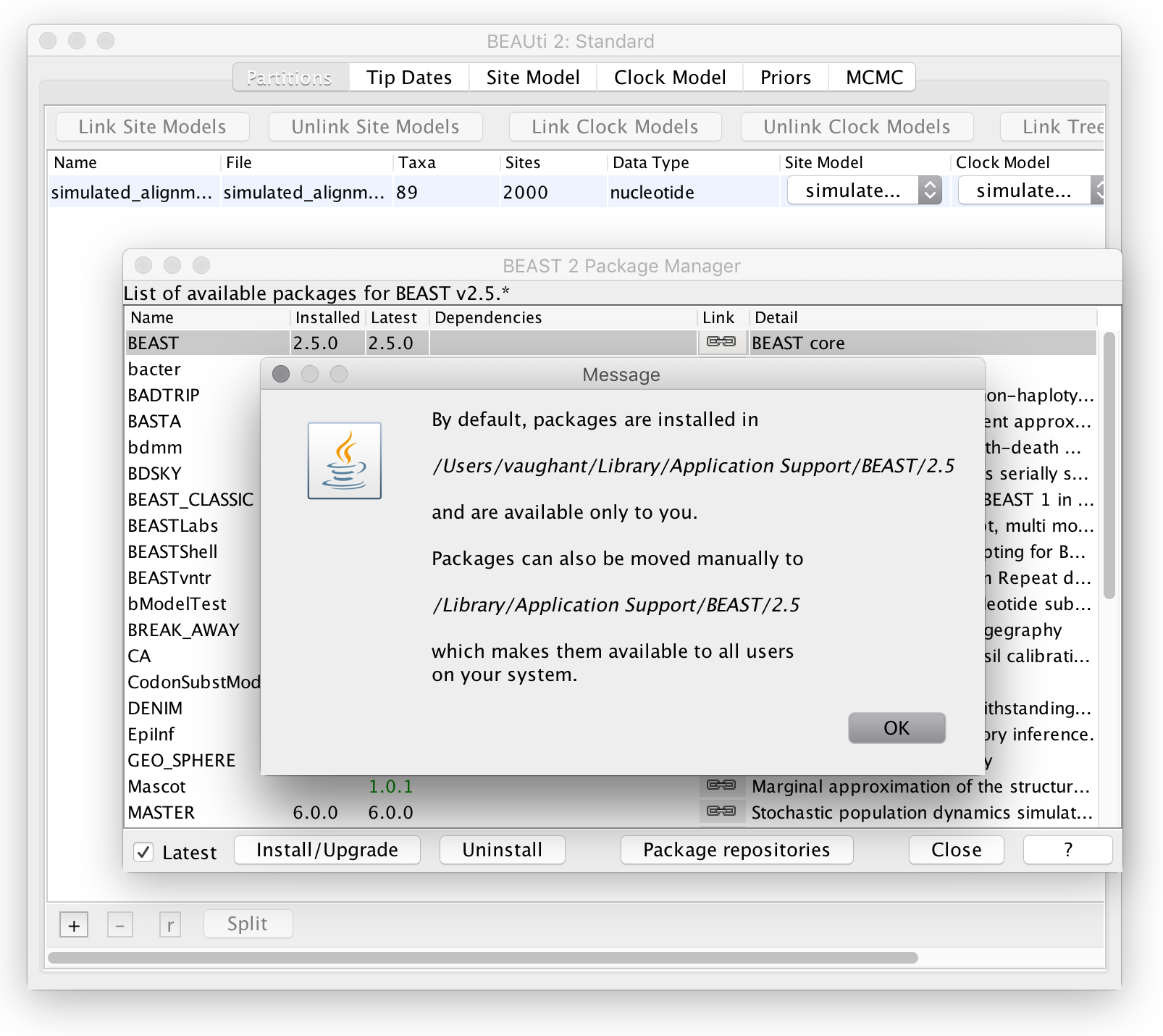
which implies that my packages are installed in

/users/vaughant/Library/Application Support/BEAST/2.5

The necessary R script can be found in the “scripts” directory within the EpiInf package directory. So on my system I can load this using the following R command:

> source("/users/vaughant/Library/Application Support/BEAST/2.5/EpiInf/scripts/plotTraj.R")

On your system the path will be different.

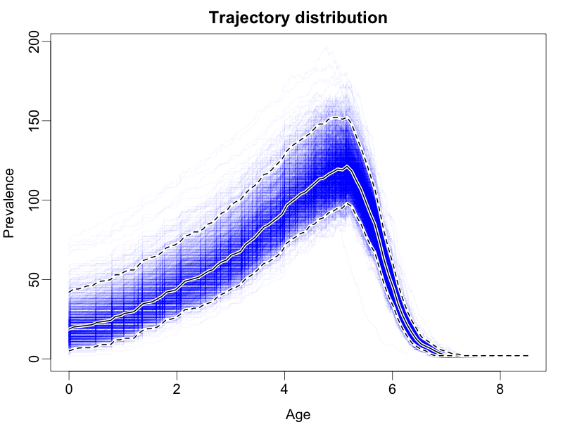
Once the script is loaded, the prevalence trajectory posterior distribution can be visualized using the following command:

plotTraj("tutorial.traj")

This should result in a figure similar to the following:

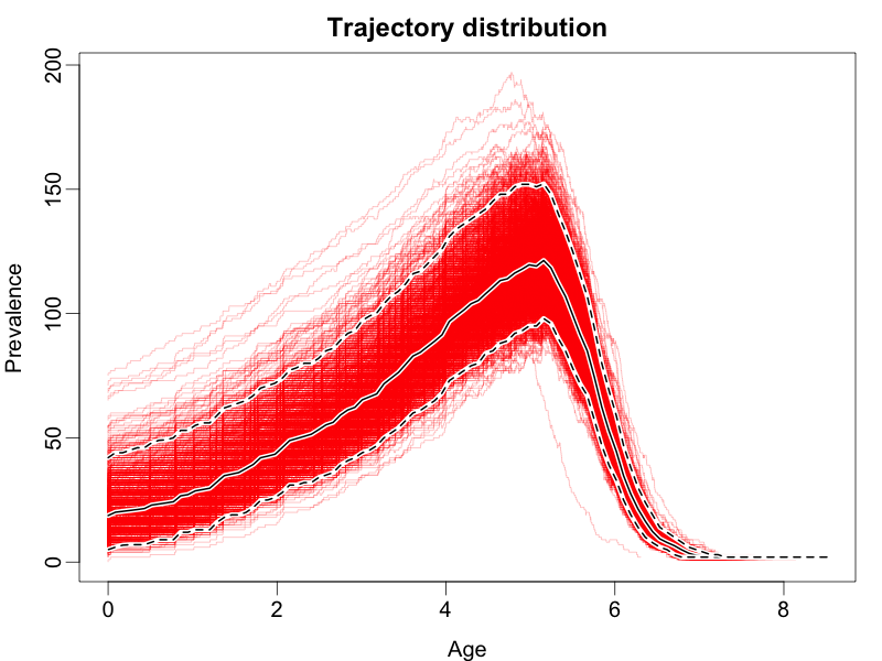
The coloured lines represent draws from the posterior, the dashed black lines represent the boundaries of the 95% highest posterior density interval for the prevalence at each time, while the solid black line represents the mean posterior prevalence.

To adjust the colour and/or opacity of the coloured lines, simply use the “col” parameter:

plotTraj("tutorial.traj", col=rgb(0,0,1,0.05))

Furthermore, the plotTraj command accepts all of the standard plot() commands such as xlim, ylim, xlab, ylab, main, log, etc.

Wrapping up

This completes the first tutorial. In a future tutorial we will demonstrate how to use EpiInf to analyze a combination of genetic and non-genetic data.