Tutorial: Basic Analysis

This tutorial will gently walk you through the process of using Bacter, from to jointly infer an ARG and population model parameters from an example multi-locus data set.

Choosing the Bacter BEAUti template

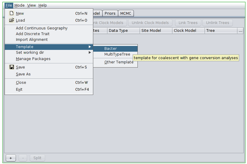
Open the BEAUti program. Before doing anything else we must switch to the Bacter template. To do this, open the file menu and from the Template submenu select “Bacter”.

Loading an alignment

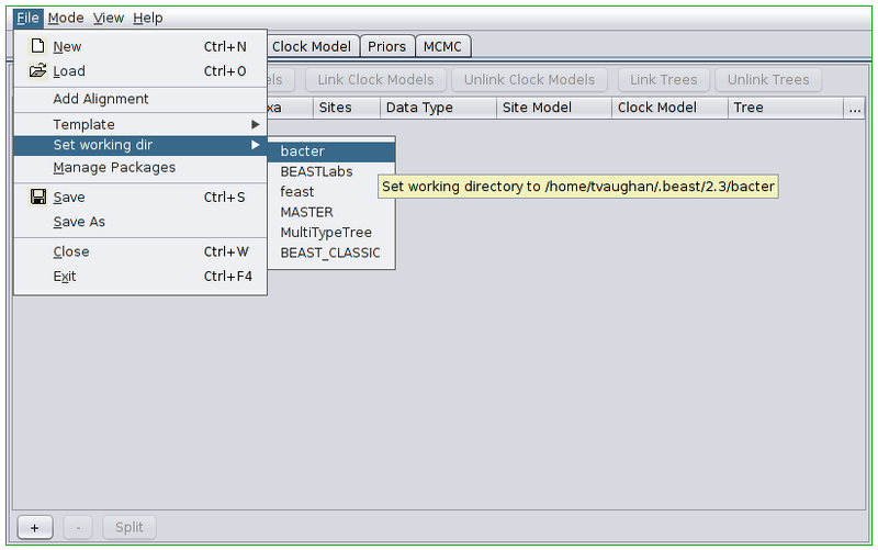
Once the appropriate template is set, we can load our sequence data. In this tutorial we will be performing an inference based on simulated data that is distributed with Bacter. To load this data, first change BEAUti’s working directory to that of the installed bacter package by selecting File->Set working dir->bacter. (This step is only useful when loading data/XMLs distributed with packages.)

Then, select File->Add Alignment, navigate to the examples/ subdirectory. Hold down the Ctrl key (or Command if you’re on a Mac) and click to select the two files simulated_data_A.fasta and simulated_data_B.fasta.

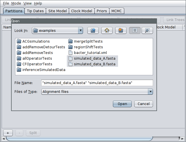
Each of these files is a simulated alignment of 20 distinct 5kb nucleotide sequences. Each file contains the multiple sequence alignment for a distinct locus. That is, each file contains exactly the same number of sequences from the same sampled bacteria but from different portions of the genome.

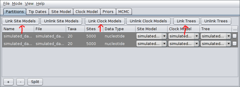
After pressing Open, the alignments should be visible as two new records in the table. By default, each locus is assumed to have its own distinct site, clock and “tree” (really ARG here) models. Since our ARGs potentially span multiple loci, we should definitely cause the loci to share a tree model. This is done by selecting both rows in the table by again holding down Ctrl (or Command) and clicking each in turn. Alternatively, you can just click on one row and then press Ctrl+A. (This is easier than clicking each row if your data consists of many loci.) Once they’re selected, press the “Link Trees” button on the right-hand side just above the table. In our case, we will use shared site and clock models too, so click the “Link Site Models” and “Link Clock Models” buttons as well.

Setting up the analysis

We will now configure the model under which the inference will be conducted.

The simulated data that we’ve loaded was sampled contemporaneously. We can therefore ignore the Tip Dates panel. When analyzing real data where the samples were collected at very different times you’ll want to include those times in the analysis by modifying the contents of that panel.

Furthermore, the data was simulated using a simple Jukes-Cantor substitution model, which is the default configuration given in the Site Model panel. When analyzing real data, you will likely want to use a more sophisticated substitution model.

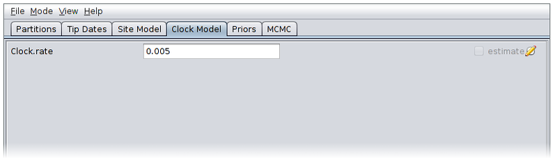
Open the Clock Model panel and set the clock rate to the true value of 0.005. (We cannot estimate this parameter without serially sampled sequence data.)

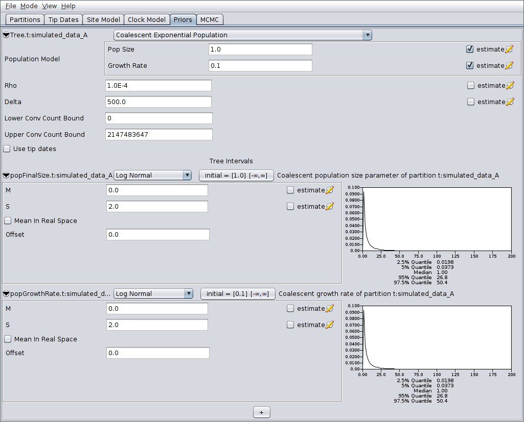
Now switch to the Priors panel. As we suspect that population which gave rise to our data was growing exponentially, select “Coalescent Exponential Population” from the drop-down list of ARG priors. Expand the tree prior by clicking on the arrow to the left of “Tree.t”.

Un-check the “estimate” checkboxes to the right of the recombination rate (Rho) and tract length (Delta) parameters and enter the values 1.0e-4 and 500.0 respectively. Estimating these parameters can actually be quite difficult, so fixing them to known values is a good idea if these are available.

Select log normal priors for the population growth rate and final size parameters, with parameters M=0 and S=2.

The priors panel should now look similar to the following:

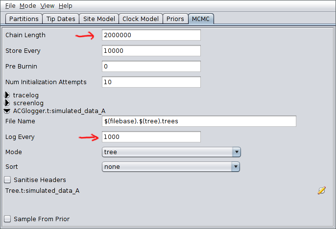
Finally, switch to the MCMC panel and change the chain length to

1. This is almost certainly far too short for a production run, but means that the example analysis will complete relatively quickly. Also, because our run is so short, we’ll sample the chain of ARGs more frequently. To do this, expand the ACGLogger.t:simulated_data_A section by clicking on the arrow to the left of this line, then set the “Log Every” field to 1000. The MCMC panel should now look similar to the following:

Once your analysis is set up, select File->Save, navigate to the directory you wish the analysis XML to be written to, give it a sensible file name (for example bacter_tutorial.xml), and press the Save button to produce the BEAST input XML.

Running the analysis

Run the analysis just as you would any other BEAST 2 analysis. That is,

1. Start BEAST 2.
2. Select the XML you produced in the previous section from the file selection dialog box.

Once BEAST is running, you should see output periodically printed to standard out (if you’re running BEAST from a terminal emulator) or the output window. The analysis we’ve set up should take around half an hour to complete on a modern computer.

Analyzing the results

During the analysis results are written to several files which can usually located in the same directory as the directory containing the input XML. These are:

1. The log file, which ends in the extension .log and contains sampled parameter values,
2. The tree file, which ends in the extension .trees and contains sampled ARGs.

Parameter posteriors

To examine the sampled parameter posteriors, open Tracer and load the log file. In our example analysis, the main parameters we’re interested in are the population growth rate and final size. The data were simulated under an exponential growth model with rate 0.5 (per unit time) and final effective size 5.0. Both these values are well within the 95% HPD intervals for the corresponding inferred parameters:

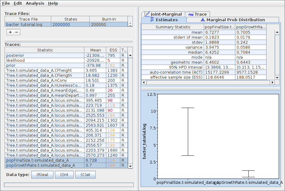
Note that the ESS for many parameters, the likelihood in particular, is still extremely small. This indicates that, as anticipated, the chain should be run for a lot longer before the results are considered trustworthy. We can easily continue/resume the chain just as for any other BEAST 2 analysis, and you may wish to try this yourself. However, in the interests of keeping the length of time needed to complete this tutorial from becoming too long, we will now proceed to further analyse the results we already have.

Viewing sampled ARGs

The ARGs sampled during a Bacter analysis can be viewed using the browser-based IcyTree phylogenetic tree and network visualizer. Beware that the viewer requires an up-to-date version of Firefox or Chrome to function correctly.

To use the viewer, simply open the IcyTree web page in a browser window, select File->“Load from file”, then choose the tree file using the file chooser. Alternatively, you can simply drag the tree file onto the IcyTree window.

Once loaded, the first ARG in the tree file is displayed. Use the comma and period (, and .) keys to step through the file one ARG at a time or the < and > keys to step in increments of 10%. Navigation can also be performed by clicking on the buttons in the lower-left corner of the window with your mouse. Further information about using IcyTree can be found by selecting items listed under the Help menu. To generate the image below, edges were coloured by locus (Style->“Colour edges by”), the colouring legend and the time axis were switched on (Style->“Display legend” and Style->“Display axis”).

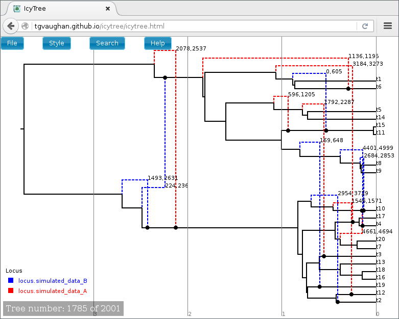
ARGs are displayed in IcyTree in a particular way. The solid lines depict lineages belonging to the clonal frame, while dashed edges representing the topology changes imposed on the clonal frame by conversions. Additional information concerning a specific edge can be viewed by hovering the mouse cursor over that edge.

It is important to remember that ARGs at the start of the file (particularly the first) will likely be very different to the true ARG, as this portion of the file represents ARGs sampled before convergence of the MCMC to the true posterior. Later trees should represent individual samples drawn from the posterior.

Creating a summary ARG

Individual ARGs sampled from the posterior are poor representations of the inference result at best, and at worst they may be completely misleading. This is because they contain no indication in the uncertainty inherent in what the sequence data tells us of the events they describe. Thus, while a single ARG sample may contain features that are well-supported by the data, the same ARG will likely contain many features that have little or no support at all.

What is needed is some kind of picture of the posterior _distribution_ over ARG space instead of a single point estimate. Unfortunately, the optimal route to producing such a summary is currently an open research question. However, Bacter provides an implementation of an algorithm for constructing a qualitative summary which is similar in spirit to the algorithms which BEAST and other Bayesian phylogenetic packages use to summarize distributions over tree space.

To produce a summary ARG, open the “AppStore” program that is distributed with BEAST 2.

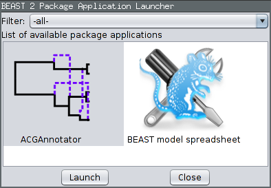
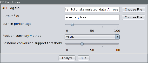
Ensure the ACGAnnotator icon is highlighted, then press the Launch button. This will open a dialog from which you can select the ACG (tree) log file and the name and location of the file to which the summary is written. In addition, you can adjust:

1. The burn-in percentage: the percentage of the tree log file which will be ignored to account for the samples that were taken before the MCMC reached convergence.
2. The position summary method: this affects the way that the internal node ages of the summary tree are chosen. The default is to use the mean of the node ages present in the sampled ARGs.
3. The posterior conversion support threshold: this is the percentage of sampled ARGs which must contain a given conversion for it to be included in the summary tree. (This is conceptually similar to the threshold for clade inclusion in a majority-rule consensus tree.)

For this tutorial, ensure the ACG (tree) log file generated by the above analysis is selected and choose summary.tree as the output file name. Leave the burn-in fraction at 10% and keep MEAN as the position summary method, but lower the conversion support threshold to 30%. This means that conversions will only have to appear in 30% of the sampled ARGs to be included in the summary. The dialog should now look like the following image:

Pressing the “Analyze” button will bring up an additional window which will report on the progress of creating the summary tree. As there are only a few hundred ARGs present in our log file, this process should only take a few seconds. Once it is complete, press the Close button. You can also exit the AppStore.

Loading the file summary.tree in IcyTree should produce something similar to the following figure. (Edges have been coloured by “locus”, the opacity of recombinant edges indicates their posterior support and they have been labelled with the sites affected by the corresponding conversion. Error bars indicating the node age 95% HPD intervals have also been included.)

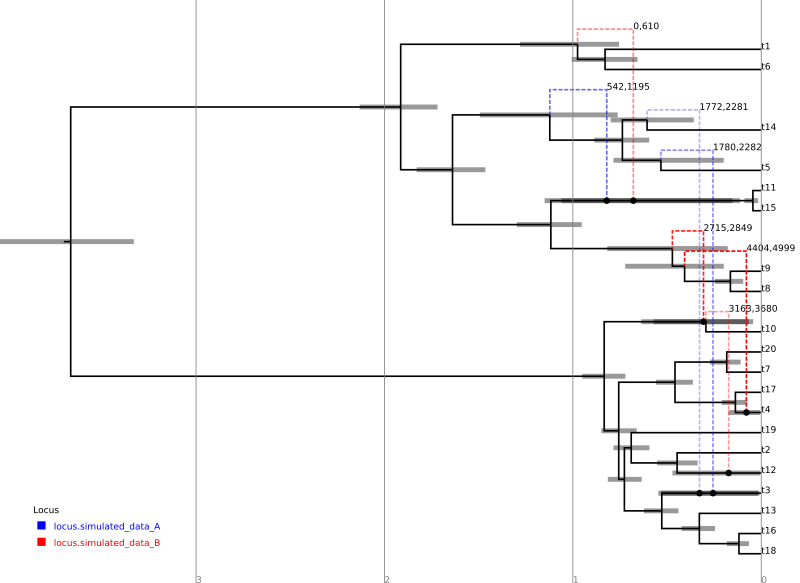
For comparison, the following depicts the true ARG that was used to produce the simulated data:

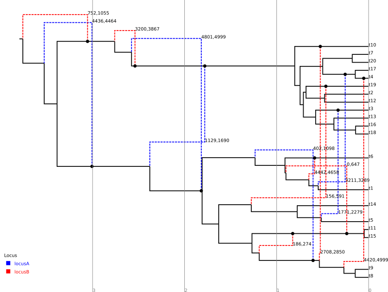
Although the inference has recovered many features of the true ARG, fewer features appear in the summary than were present in reality. This is a side-effect of the summary procedure, which includes only those features that have adequate support. Features in the original which did not produce a strong signal in the data do not appear in the summary. In addition, since the chain has not completely converged to the true posterior, running the algorithm for more steps will no-doubt recover a greater fraction of the conversions.

In addition, notice the pair of low-support conversions between the clonal frame edges above leaf nodes t3 and t5/t14. These edges correspond to almost precisely the same sites on locus A. These two conversions actually represent uncertainty in the source edge of a single conversion coming from either t5 or t14 to arrive at t3. (From the true ARG we see that the fragment actually comes from t5.) It is important to be aware of this artifact of the summary procedure. Even if a single connection point of a recombinant edge is known with a high degree of confidence, uncertainty in the location of the other point may cause the conversion to appear as a number of lower-support edges.

Wrapping up

This completes the first tutorial. In a future tutorial we will demonstrate how to use Bacter to perform non-parametric inference of population dynamics (Bayesian Skyline Plots from ARGs).