3Hamiltonian Mechanics
Numerical experiments are just what their name implies: experiments. In describing and evaluating them, one should enter the state of mind of the experimental physicist, rather than that of the mathematician. Numerical experiments cannot be used to prove theorems; but, from the physicist's point of view, they do often provide convincing evidence for the existence of a phenomenon. We will therefore follow an informal, descriptive and non-rigorous approach. Briefly stated, our aim will be to understand the fundamental properties of dynamical systems rather than to prove them.
Michel Hénon, “Numerical Exploration of Hamiltonian Systems,” in Chaotic Behavior of Deterministic Systems [21], p. 57.
The formulation of mechanics with generalized coordinates and momenta as dynamical state variables is called the Hamiltonian formulation. The Hamiltonian formulation of mechanics is equivalent to the Lagrangian formulation; however, each presents a useful point of view. The Lagrangian formulation is especially useful in the initial formulation of a system. The Hamiltonian formulation is especially useful in understanding the evolution of a system, especially when there are symmetries and conserved quantities.
For each continuous symmetry of a mechanical system there is a conserved quantity. If the generalized coordinates can be chosen to reflect a symmetry, then, by the Lagrange equations, the momenta conjugate to the cyclic coordinates are conserved. We have seen that such conserved quantities allow us to deduce important properties of the motion. For instance, consideration of the energy and angular momentum allowed us to deduce that rotation of a free rigid body about the axis of intermediate moment of inertia is unstable, and that rotation about the other principal axes is stable. For the axisymmetric top, we used two conserved momenta to reexpress the equations governing the evolution of the tilt angle so that they involve only the tilt angle and its derivative. The evolution of the tilt angle can be determined independently and has simply periodic solutions. Consideration of the conserved momenta has provided key insight. The Hamiltonian formulation is motivated by the desire to focus attention on the momenta.
In the Lagrangian formulation the momenta are, in a sense, secondary quantities: the momenta are functions of the state space variables, but the evolution of the state space variables depends on the state space variables and not on the momenta. To make use of any conserved momenta requires fooling around with the specific equations. The momenta can be rewritten in terms of the coordinates and the velocities, so, locally, we can solve for the velocities in terms of the coordinates and momenta. For a given mechanical system, and a Lagrangian describing its dynamics in a given coordinate system, the momenta and the velocities can be deduced from each other. Thus we can represent the dynamical state of the system in terms of the coordinates and momenta just as well as with the coordinates and the velocities. If we use the coordinates and momenta to represent the state and write the associated state derivative in terms of the coordinates and momenta, then we have a self-contained system. This formulation of the equations governing the evolution of the system has the advantage that if some of the momenta are conserved, the remaining equations are immediately simplified.
The Lagrangian formulation of mechanics has provided the means to investigate the motion of complicated mechanical systems. We have found that dynamical systems exhibit a bewildering variety of possible motions. The motion is sometimes rather simple and sometimes very complicated. Sometimes the evolution is very sensitive to the initial conditions, and sometimes it is not. And sometimes there are orbits that maintain resonance relationships with a drive. Consider the periodically driven pendulum: it can behave more or less as an undriven pendulum with extra wiggles, it can move in a strongly chaotic manner, or it can move in resonance with the drive, oscillating once for every two cycles of the drive or looping around once per drive cycle. Or consider the Moon. The Moon rotates synchronously with its orbital motion, always pointing roughly the same face to the Earth. However, Mercury rotates three times every two times it circles the Sun, and Hyperion rotates chaotically.
How can we make sense of this? How do we put the possible motions of these systems in relation to one another? What other motions are possible? The Hamiltonian formulation of dynamics provides a convenient framework in which the possible motions may be placed and understood. We will be able to see the range of stable resonance motions and the range of states reached by chaotic trajectories, and discover other unsuspected possible motions. So the Hamiltonian formulation gives us much more than the stated goal of expressing the system derivative in terms of potentially conserved quantities.
3.1 Hamilton's Equations
The momenta are given by momentum state functions of the time, the coordinates, and the velocities.1 Locally, we can find inverse functions that give the velocities in terms of the time, the coordinates, and the momenta. We can use this inverse function to represent the state in terms of the coordinates and momenta rather than the coordinates and velocities. The equations of motion when recast in terms of coordinates and momenta are called Hamilton's canonical equations.
We present three derivations of Hamilton's equations. The first derivation is guided by the strategy outlined above and uses nothing more complicated than implicit functions and the chain rule. The second derivation (section 3.1.1) first abstracts a key part of the first derivation and then applies the more abstract machinery to derive Hamilton's equations. The third (section 3.1.2) uses the action principle.
Lagrange's equations give us the time derivative of the momentum p on a path q:
where
To eliminate Dq we need to solve equation (3.2) for Dq in terms of p.
Let
then
So
The Lagrange equation (3.1) can be rewritten in terms of p using
We can also use
Equations (3.7) and (3.8) give the rate of change of q and p along realizable paths as functions of t, q, and p along the paths.
Though these equations fulfill our goal of expressing the equations of motion entirely in terms of coordinates and momenta, we can find a better representation. Define the function
which is the Lagrangian reexpressed as a function of time, coordinates, and momenta.2 For the equations of motion we need ∂1L evaluated with the appropriate arguments. Consider
where we used the chain rule in the first step and the inverse property (3.6) of
where the Hamiltonian H is defined by4
Using the algebraic result (3.11), the Lagrange equation (3.7) for Dp becomes
The equation for Dq can also be written in terms of H. Consider
To carry out the derivative of
again using the inverse property (3.6) of
Using the algebraic result (3.16), equation (3.8) for Dq becomes
Equations (3.13) and (3.17) give the derivatives of the coordinate and momentum path functions at each time in terms of the time, and the coordinates and momenta at that time. These equations are known as Hamilton's equations:5
The first equation is just a restatement of the relationship of the momenta to the velocities in terms of the Hamiltonian and holds for any path, whether or not it is a realizable path. The second equation holds only for realizable paths.
Hamilton's equations have an especially simple and symmetrical form. Just as Lagrange's equations are constructed from a real-valued function, the Lagrangian, Hamilton's equations are constructed from a real-valued function, the Hamiltonian. The Hamiltonian function is6
The Hamiltonian has the same value as the energy function ℰ (see equation 1.142), except that the velocities are expressed in terms of time, coordinates, and momenta by
Illustration
Let's try something simple: the motion of a particle of mass m with potential energy V (x, y). A Lagrangian is
To form the Hamiltonian we find the momenta p = ∂2L(t, q, v): px = mvx and py = mvy. Solving for the velocities in terms of the momenta is easy here:
The kinetic energy is a homogeneous quadratic form in the velocities, so the energy is T + V and the Hamiltonian is the energy expressed in terms of momenta rather than velocities. Hamilton's equations for Dq are
Note that these equations merely restate the relation between the momenta and the velocities. Hamilton's equations for Dp are
The rate of change of the linear momentum is minus the gradient of the potential energy.
Exercise 3.1: Deriving Hamilton's equations
For each of the following Lagrangians derive the Hamiltonian and Hamilton's equations. These problems are simple enough to do by hand.
a. A Lagrangian for a planar pendulum:
b. A Lagrangian for a particle of mass m with a two-dimensional potential energy V(x, y) = (x2 + y2)/2 + x2y − y3/3 is
c. A Lagrangian for a particle of mass m constrained to move on a sphere of radius
Exercise 3.2: Sliding pendulum
For the pendulum with a sliding support (see exercise 1.20), derive a Hamiltonian and Hamilton's equations.
Hamiltonian state
Given a coordinate path q and a Lagrangian L, the corresponding momentum path p is given by equation (3.2). Equation (3.17) expresses the same relationship in terms of the corresponding Hamiltonian H. That these relations are valid for any path, whether or not it is a realizable path, allows us to abstract to arbitrary velocity and momentum at a moment. At a moment, the momentum p for the state tuple (t, q, v) is p = ∂2L(t, q, v). We also have v = ∂2H(t, q, p). In the Lagrangian formulation the state of the system at a moment can be specified by the local state tuple (t, q, v) of time, generalized coordinates, and generalized velocities. Lagrange's equations determine a unique path emanating from this state. In the Hamiltonian formulation the state can be specified by the tuple (t, q, p) of time, generalized coordinates, and generalized momenta. Hamilton's equations determine a unique path emanating from this state. The Lagrangian state tuple (t, q, v) encodes exactly the same information as the Hamiltonian state tuple (t, q, p); we need a Lagrangian or a Hamiltonian to relate them. The two formulations are equivalent in that the same coordinate path emanates from them for equivalent initial states.
The Lagrangian state derivative is constructed from the Lagrange equations by solving for the highest-order derivative and abstracting to arbitrary positions and velocities at a moment.7 The Lagrangian state path is generated by integration of the Lagrangian state derivative given an initial Lagrangian state (t, q, v). Similarly, the Hamiltonian state derivative can be constructed from Hamilton's equations by abstracting to arbitrary positions and momenta at a moment. Hamilton's equations are a set of first-order differential equations in explicit form. The Hamiltonian state derivative can be directly written in terms of them. The Hamiltonian state path is generated by integration of the Hamiltonian state derivative given an initial Hamiltonian state (t, q, p). If these state paths are obtained by integrating the state derivatives with equivalent initial states, then the coordinate path components of these state paths are the same and satisfy the Lagrange equations. The coordinate path and the momentum path components of the Hamiltonian state path satisfy Hamilton's equations. The Hamiltonian formulation and the Lagrangian formulation are equivalent.
Given a path q, the Lagrangian state path and the Hamiltonian state paths can be deduced from it. The Lagrangian state path Γ[q] can be constructed from a path q simply by taking derivatives. The Lagrangian state path satisfies:
The Lagrangian state path is uniquely determined by the path q. The Hamiltonian state path ΠL[q] can also be constructed from the path q but the construction requires a Lagrangian. The Hamiltonian state path satisfies
The Hamiltonian state tuple is not uniquely determined by the path q because it depends upon our choice of Lagrangian, which is not unique.
The 2n-dimensional space whose elements are labeled by the n generalized coordinates qi and the n generalized momenta pi is called the phase space. The components of the generalized coordinates and momenta are collectively called the phase-space components.8 The dynamical state of the system is completely specified by the phase-space state tuple (t, q, p), given a Lagrangian or Hamiltonian to provide the map between velocities and momenta.
Computing Hamilton's equations
Hamilton's equations are a system of first-order ordinary differential equations. A procedural formulation of Lagrange's equations as a first-order system was presented in section 1.7. The following formulation of Hamilton's equations is analogous:
(define ((Hamilton-equations Hamiltonian) q p)
  (let ((state-path (qp->H-state-path q p)))
    (- (D state-path)
       (compose (Hamiltonian->state-derivative Hamiltonian)
                state-path))))
The Hamiltonian state derivative is computed as follows:
(define ((Hamiltonian->state-derivative Hamiltonian) H-state)
  (up 1
      (((partial 2) Hamiltonian) H-state)
      (- (((partial 1) Hamiltonian) H-state))))
The state in the Hamiltonian formulation is composed of the time, the coordinates, and the momenta. We call this an H-state, to distinguish it from the state in the Lagrangian formulation. We can select the components of the Hamiltonian state with the selectors time, coordinate, momentum. We construct Hamiltonian states from their components with up. The first component of the state is time, so the first component of the state derivative is one, the time rate of change of time. Given procedures q and p implementing coordinate and momentum path functions, the Hamiltonian state path can be constructed with the following procedure:
(define ((qp->H-state-path q p) t)
  (up t (q t) (p t)))
The Hamilton-equations procedure returns the residuals of Hamilton's equations for the given paths.
For example, a procedure implementing the Hamiltonian for a point mass with potential energy V (x, y) is
(define ((H-rectangular m V) state)
  (let ((q (coordinate state))
        (p (momentum state)))
    (+ (/ (square p) (* 2 m))
       (V (ref q 0) (ref q 1)))))
Hamilton's equations are
(show-expression
  (let ((V (literal-function 'V (-> (X Real Real) Real)))
        (q (up (literal-function 'x)
               (literal-function 'y)))
        (p (down (literal-function 'p_x)
                 (literal-function 'p_y))))
(((Hamilton-equations (H-rectangular 'm V)) q p) 't)))The zero in the first element of the structure of Hamilton's equation residuals is just the tautology that time advances uniformly: the time function is just the identity, so its derivative is one and the residual is zero. The equations in the second element of the structure relate the coordinate paths and the momentum paths. The equations in the third element give the rate of change of the momenta in terms of the applied forces.
Exercise 3.3: Computing Hamilton's equations
Check your answers to exercise 3.1 with the Hamilton-equations procedure.
3.1.1 The Legendre Transformation
The Legendre transformation abstracts a key part of the process of transforming from the Lagrangian to the Hamiltonian formulation of mechanics—the replacement of functional dependence on generalized velocities with functional dependence on generalized momenta. The momentum state function is defined as a partial derivative of the Lagrangian, a real-valued function of time, coordinates, and velocities. The Legendre transformation provides an inverse that gives the velocities in terms of the momenta: we are able to write the velocities as a partial derivative of a different real-valued function of time, coordinates, and momenta.9
Given a real-valued function F, if we can find a real-valued function G such that DF = (DG)−1, then we say that F and G are related by a Legendre transform.
Locally, we can define the inverse function10
Since
we have
or
The integral is determined up to a constant of integration. If we define
then we have
The function G has the desired property that DG is the inverse function
Given a relation w = DF (v) for some given function F, then v = DG(w) for
A picture may help (see figure 3.1). The curve is the graph of the function DF. Turned sideways, it is also the graph of the function DG, because DG is the inverse function of DF. The integral of DF from v0 to v is F(v) − F(v0); this is the area below the curve from v0 to v. Likewise, the integral of DG from w0 to w is G(w) − G(w0); this is the area to the left of the curve from w0 to w. The union of these two regions has area wv − w0v0. So
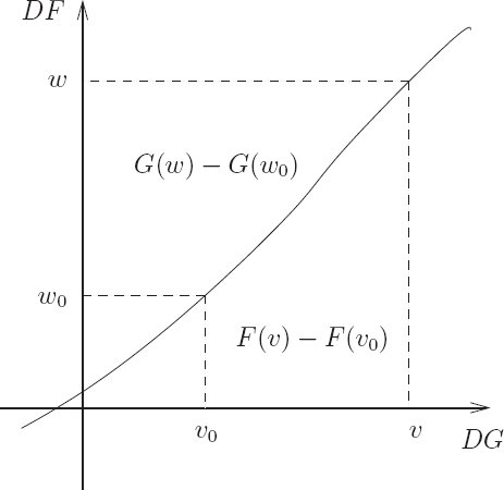
which is the same as
The left-hand side depends only on the point labeled by w and v and the right-hand side depends only on the point labeled by w0 and v0, so these must be constant, independent of the variable endpoints. So as the point is changed the combination G(w) + F(v) − wv is invariant. Thus
with constant C. The requirement for G depends only on DG so we can choose to define G with C = 0.
Legendre transformations with passive arguments
Let F be a real-valued function of two arguments and
If we can find a real-valued function G such that
we say that F and G are related by a Legendre transformation, that the second argument in each function is active, and that the first argument is passive in the transformation.
If the function ∂1F can be locally inverted with respect to the second argument we can define
giving
where W = I1 is the selector function for the second argument.
For the active arguments the derivation goes through as before. The first argument to F and G is just along for the ride—it is a passive argument. Let
then define
We can check that G has the property
but
or
So, from equation (3.42),
as required. The active argument may have many components.
The partial derivatives with respect to the passive arguments are related in a remarkably simple way. Let's calculate the derivative ∂0G in pieces. First,
because ∂0W = 0. We calculate
Putting these together, we find
The calculation is unchanged if the passive argument has many components.
We can write the Legendre transformation more symmetrically:
The last relation is not as trivial as it looks, because x enters the equations connecting w and v. With this symmetrical form, we see that the Legendre transform is its own inverse.
Exercise 3.4: Simple Legendre transforms
For each of the following functions, find the function that is related to the given function by the Legendre transform on the indicated active argument. Show that the Legendre transform relations hold for your solution, including the relations among passive arguments, if any.
a. F (x) = ax + bx2, with no passive arguments.
b. F (x, y) = a sin x cos y, with x active.
c. F (x, y, ẋ, ẏ) = xẋ2 + 3ẋẏ + yẏ2, with ẋ and ẏ active.
Hamilton's equations from the Legendre transformation
We can use the Legendre transformation with the Lagrangian playing the role of F and with the generalized velocity slot playing the role of the active argument. The Hamiltonian plays the role of G with the momentum slot active. The coordinate and time slots are passive arguments.
The Lagrangian L and the Hamiltonian H are related by a Legendre transformation:
and
with passive equations
Presuming it exists, we can define the inverse of ∂2L with respect to the last argument:
and write the Hamiltonian
These relations are purely algebraic in nature.
On a path q we have the momentum p:
and from the definition of
The Legendre transform gives
This relation is purely algebraic and is valid for any path. The passive equation (3.54) gives
but the left-hand side can be rewritten using the Lagrange equations, so
This equation is valid only for realizable paths, because we used the Lagrange equations to derive it. Equations (3.59) and (3.61) are Hamilton's equations.
The remaining passive equation is
This passive equation says that the Lagrangian has no explicit time dependence (∂0L = 0) if and only if the Hamiltonian has no explicit time dependence (∂0H = 0). We have found that if the Lagrangian has no explicit time dependence, then energy is conserved. So if the Hamiltonian has no explicit time dependence then it is a conserved quantity.
Exercise 3.5: Conservation of the Hamiltonian
Using Hamilton's equations, show directly that the Hamiltonian is a conserved quantity if it has no explicit time dependence.
Legendre transforms of quadratic functions
We cannot implement the Legendre transform in general because it involves finding the functional inverse of an arbitrary function. However, many physical systems can be described by Lagrangians that are quadratic forms in the generalized velocities. For such functions the generalized momenta are linear functions of the generalized velocities, and thus explicitly invertible.
More generally, we can compute a Legendre transformation for polynomial functions where the leading term is a quadratic form:
Because the first term is a quadratic form only the symmetric part of M contributes to the result, so we can assume M is symmetric.12 Let w = DF (v), then
So if M is invertible we can solve for v in terms of w. Thus we may define a function
and we can use this to compute the value of the function G:
Computing Hamiltonians
We implement the Legendre transform for quadratic functions by the procedure13
(define (Legendre-transform F)
  (let ((w-of-v (D F)))
    (define (G w)
      (let ((zero (compatible-zero w)))
        (let ((M ((D w-of-v) zero))
              (b (w-of-v zero)))
          (let ((v (solve-linear-left M (- w b))))
            (- (* w v) (F v))))))
    G))
The procedure Legendre-transform takes a procedure of one argument and returns the procedure that is associated with it by the Legendre transform. If w = DF (v), wv = F (v) + G(w), and v = DG(w) specifies a one-argument Legendre transformation, then G is the function associated with F by the Legendre transform:
We can use the Legendre-transform procedure to compute a Hamiltonian from a Lagrangian:
(define ((Lagrangian->Hamiltonian Lagrangian) H-state)
  (let ((t (time H-state))
        (q (coordinate H-state))
        (p (momentum H-state)))
    (define (L qdot)
      (Lagrangian (up t q qdot)))
    ((Legendre-transform L) p)))
Notice that the one-argument Legendre-transform procedure is sufficient. The passive variables are given no special attention, they are just passed around.
The Lagrangian may be obtained from the Hamiltonian by the procedure:
(define ((Hamiltonian->Lagrangian Hamiltonian) L-state)
  (let ((t (time L-state))
        (q (coordinate L-state))
        (qdot (velocity L-state)))
    (define (H p)
      (Hamiltonian (up t q p)))
    ((Legendre-transform H) qdot)))
Notice that the two procedures Hamiltonian->Lagrangian and Lagrangian->Hamiltonian are identical, except for the names.
For example, the Hamiltonian for the motion of the point mass with the potential energy V (x, y) may be computed from the Lagrangian:
(define ((L-rectangular m V) local)
  (let ((q (coordinate local))
        (qdot (velocity local)))
    (- (* 1/2 m (square qdot))
       (V (ref q 0) (ref q 1)))))
And the Hamiltonian is, as we saw in equation (3.22):
(show-expression
  ((Lagrangian->Hamiltonian
     (L-rectangular
       'm
       (literal-function 'V (-> (X Real Real) Real))))
   (up 't (up 'x 'y) (down 'p_x 'p_y))))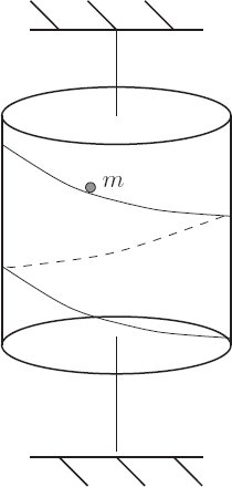
Exercise 3.6: On a helical track
A uniform cylinder of mass M, radius R, and height h is mounted so as to rotate freely on a vertical axis. A point mass of mass m is constrained to move on a uniform frictionless helical track of pitch β (measured in radians per meter of drop along the cylinder) mounted on the surface of the cylinder (see figure 3.2). The mass is acted upon by standard gravity (g = 9.8 ms−2).
a. What are the degrees of freedom of this system? Pick and describe a convenient set of generalized coordinates for this problem. Write a Lagrangian to describe the dynamical behavior. It may help to know that the moment of inertia of a cylinder around its axis is
b. Make a Hamiltonian for the system. Write Hamilton's equations for the system. Are there any conserved quantities?
c. If we release the point mass at time t = 0 at the top of the track with zero initial speed and let it slide down, what is the motion of the system?
Exercise 3.7: An ellipsoidal bowl
Consider a point particle of mass m constrained to move in a bowl and acted upon by a uniform gravitational acceleration g. The bowl is ellipsoidal, with height z = ax2 + by2. Make a Hamiltonian for this system. Can you make any immediate deductions about this system?
3.1.2 Hamilton's Equations from the Action Principle
The previous two derivations of Hamilton's equations made use of the Lagrange equations. Hamilton's equations can also be derived directly from the action principle.
The action is the integral of the Lagrangian along a path:
The action is stationary with respect to variations of a realizable path that preserve the configuration at the endpoints (for Lagrangians that are functions of time, coordinates, and velocities).
We can rewrite the integrand in terms of the Hamiltonian
with p(t) = ∂2L(t, q(t), Dq(t)). The Legendre transformation construction gives
which is one of Hamilton's equations, the one that does not depend on the path being a realizable path.
In order to vary the action we should make the dependences on the path explicit. We introduce
and14
The integrand of the action integral is then
Using the shorthand δp for
Integrating the second term by parts, using D(pδq) = Dpδq + pDδq, we get
The variations are constrained so that δq(t1) = δq(t2) = 0, so the integrated part vanishes. Rearranging terms, the variation of the action is
As a consequence of equation (3.69), the factor multiplying δp is zero. We are left with
For the variation of the action to be zero for arbitrary variations, except for the endpoint conditions, we must have
or
which is the “dynamical” Hamilton equation.16
3.1.3 A Wiring Diagram
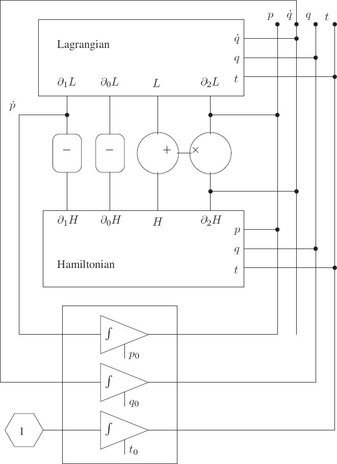
Figure 3.3 shows a summary of the functional relationship between the Lagrangian and the Hamiltonian descriptions of a dynamical system. The diagram shows a “circuit” interconnecting some “devices” with “wires.” The devices represent the mathematical functions that relate the quantities on their terminals. The wires represent identifications of the quantities on the terminals that they connect. For example, there is a box that represents the Lagrangian function. Given values t, q, and
The upper part of the diagram summarizes the relationship of the Hamiltonian to the Lagrangian. For example, the sum of the values on the terminals L of the Lagrangian and H of the Hamiltonian is the product of the value on the
One can use this diagram to help understand the underlying unity of the Lagrangian and Hamiltonian formulations of mechanics. Lagrange's equations are just the connection of the ṗ wire to the ∂1L terminal of the Lagrangian device. One of Hamilton's equations is just the connection of the ṗ wire (through the negation device) to the ∂1H terminal of the Hamiltonian device. The other is just the connection of the
3.2 Poisson Brackets
Here we introduce the Poisson bracket, in terms of which Hamilton's equations have an elegant and symmetric expression. Consider a function F of time, coordinates, and momenta. The value of F along the path σ(t) = (t, q(t), p(t)) is (F ∘ σ)(t) = F (t, q(t), p(t)). The time derivative of F ∘ σ is
If the phase-space path is a realizable path for a system with Hamiltonian H, then Dq and Dp can be reexpressed using Hamilton's equations:
where the Poisson bracket {F, H} of F and H is defined by17
Note that the Poisson bracket of two functions on the phase-state space is also a function on the phase-state space.
The coordinate selector Q = I1 is an example of a function on phase-state space: Q(t, q, p) = q. According to equation (3.80),
but this is the same as Hamilton's equation
Similarly, the momentum selector P = I2 is a function on phase-state space: P (t, q, p) = p. We have
which is the same as Hamilton's other equation
So the Poisson bracket provides a uniform way of writing Hamilton's equations:
The Poisson bracket of any function with itself is zero, so we recover the conservation of energy for a system that has no explicit time dependence:
Properties of the Poisson bracket
Let F, G, and H be functions of time, position, and momentum, and let c be independent of position and momentum.
The Poisson bracket is antisymmetric:
It is bilinear (linear in each argument):
The Poisson bracket satisfies Jacobi's identity:
All but the last of (3.88–3.93) can immediately be verified from the definition. Jacobi's identity requires a little more effort to verify. We can use the computer to avoid some work. Define some literal phase-space functions of Hamiltonian type:
(define F
  (literal-function 'F
                    (-> (UP Real (UP Real Real) (DOWN Real Real)) Real)))

(define G
  (literal-function 'G
                    (-> (UP Real (UP Real Real) (DOWN Real Real)) Real)))

(define H
  (literal-function 'H
                    (-> (UP Real (UP Real Real) (DOWN Real Real)) Real)))
Then we check the Jacobi identity:
((+ (Poisson-bracket F (Poisson-bracket G H))
    (Poisson-bracket G (Poisson-bracket H F))
    (Poisson-bracket H (Poisson-bracket F G)))
(up 't (up 'x 'y) (down 'px 'py)))0The residual is zero, so the Jacobi identity is satisfied for any three phase-space state functions with two degrees of freedom.
Poisson brackets of conserved quantities
The Poisson bracket of conserved quantities is conserved. Let F and G be time-independent phase-space state functions: ∂0F = ∂0G = 0. If F and G are conserved by the evolution under H then
So the Poisson brackets of F and G with H are zero: {F, H} = {G, H} = 0. The Jacobi identity then implies
and thus
so {F, G} is a conserved quantity. The Poisson bracket of two conserved quantities is also a conserved quantity.
3.3 One Degree of Freedom
The solutions of time-independent systems with one degree of freedom can be found by quadrature. Such systems conserve the Hamiltonian: the Hamiltonian has a constant value on each realizable trajectory. We can use this constraint to eliminate the momentum in favor of the coordinate, obtaining the single equation Dq(t) = f(q(t)).18
A geometric view reveals more structure. Time-independent systems with one degree of freedom have a two-dimensional phase space. Energy is conserved, so all orbits are level curves of the Hamiltonian. The possible orbit types are restricted to curves that are contours of a real-valued function. The possible orbits are paths of constant altitude in the mountain range on the phase plane described by the Hamiltonian.
Only a few characteristic features are possible. There are points that are stable equilibria of the dynamical system. These are the peaks and pits of the Hamiltonian mountain range. These equilibria are stable in the sense that neighboring trajectories on nearby contours stay close to the equilibrium point. There are orbits that trace simple closed curves on contours that surround a peak or pit, or perhaps several peaks. There are also trajectories lying on contours that cross at a saddle point. The crossing point is an unstable equilibrium, unstable in the sense that neighboring trajectories leave the vicinity of the equilibrium point. Such contours that cross at saddle points are called separatrices (singular: separatrix), contours that “separate” two regions of distinct behavior.
At every point Hamilton's equations give a unique rate of evolution and direct the system to move perpendicular to the gradient of the Hamiltonian. At the peaks, pits, and saddle points, the gradient of the Hamiltonian is zero, so according to Hamilton's equations these are equilibria. At other points, the gradient of the Hamiltonian is nonzero, so according to Hamilton's equations the rate of evolution is nonzero. Trajectories evolve along the contours of the Hamiltonian. Trajectories on simple closed contours periodically trace the contour. At a saddle point, contours cross. The gradient of the Hamiltonian is zero at the saddle point, so a system started at the saddle point does not leave the saddle point. On the separatrix away from the saddle point the gradient of the Hamiltonian is not zero, so trajectories evolve along the contour. Trajectories on the separatrix are asymptotic forward or backward in time to a saddle point. Going forward or backward in time, such trajectories forever approach an unstable equilibrium but never reach it. If the phase space is bounded, asymptotic trajectories that lie on contours of a smooth Hamiltonian are always asymptotic to unstable equilibria at both ends (but they may be different equilibria).
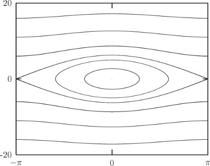
These orbit types are all illustrated by the prototypical phase plane of the pendulum (see figure 3.4). The solutions lie on contours of the Hamiltonian. There are three regions of the phase plane; in each the motion is qualitatively different. In the central region the pendulum oscillates; above this there is a region in which the pendulum circulates in one direction; below the oscillation region the pendulum circulates in the other direction. In the center of the oscillation region there is a stable equilibrium, at which the pendulum is hanging motionless. At the boundaries between these regions, the pendulum is asymptotic to the unstable equilibrium, at which the pendulum is standing upright.19 There are two asymptotic trajectories, corresponding to the two ways the equilibrium can be approached. Each of these is also asymptotic to the unstable equilibrium going backward in time.
3.4 Phase Space Reduction
Our motivation for the development of Hamilton's equations was to focus attention on the quantities that can be conserved—the momenta and the energy. In the Hamiltonian formulation the generalized configuration coordinates and the conjugate momenta comprise the state of the system at a given time. We know from the Lagrangian formulation that if the Lagrangian does not depend on some coordinate then the conjugate momentum is conserved. This is also true in the Hamiltonian formulation, but there is a distinct advantage to the Hamiltonian formulation. In the Lagrangian formulation the knowledge of the conserved momentum does not lead immediately to any simplification of the problem, but in the Hamiltonian formulation the fact that momenta are conserved gives an immediate reduction in the dimension of the system to be solved. In fact, if a coordinate does not appear in the Hamiltonian then the dimension of the system of coupled equations that remain to be solved is reduced by two—the coordinate does not appear and the conjugate momentum is constant.
Let H(t, q, p) be a Hamiltonian for some problem with an n-dimensional configuration space and 2n-dimensional phase space. Suppose the Hamiltonian does not depend upon the ith coordinate qi: (∂1H)i = 0.20 According to Hamilton's equations, the conjugate momentum pi is conserved. Hamilton's equations of motion for the remaining 2n − 2 phase-space variables do not involve qi (because it does not appear in the Hamiltonian), and pi is a constant. Thus the dimension of the difficult part of the problem, the part that involves the solution of coupled ordinary differential equations, is reduced by two. The remaining equation governing the evolution of qi in general depends on all the other variables, but once the reduced problem has been solved, the equation of motion for qi can be written so as to give Dqi explicitly as a function of time. We can then find qi as a definite integral of this function.21
Contrast this result with analogous results for more general systems of differential equations. There are two independent situations. One situation is that we know a constant of the motion. In general, constants of the motion can be used to reduce by one the dimension of the unsolved part of the problem. To see this, let the system of equations be
where m is the dimension of the system. Assume we know some constant of the motion
At least locally, we expect that we can use this equation to solve for zm−1(t) in terms of all the other variables, and use this solution to eliminate the dependence on zm−1(t). The first m−1 equations then depend only upon the first m − 1 variables. The dimension of the system of equations to be solved is reduced by one. After the solution for the other variables has been found, zm−1(t) can be found using the constant of the motion.
The second situation is that one of the variables, say zi, does not appear in the equations of motion (but there is an equation for Dzi). In this case the equations for the other variables form an independent set of equations of one dimension less than the original system. After these are solved, then the remaining equation for zi can be solved by definite integration.
In both situations the dimension of the system of coupled equations is reduced by one. Hamilton's equations are different in that these two situations come together. If a Hamiltonian for a system does not depend on a particular coordinate, then the equations of motion for the other coordinates and momenta do not depend on that coordinate. Furthermore, the momentum conjugate to that coordinate is a constant of the motion. An added benefit is that the use of this constant of the motion to reduce the dimension of the remaining equations is automatic in the Hamiltonian formulation. The conserved momentum is a state variable and just a parameter in the remaining equations.
So if there is a continuous symmetry it will probably be to our advantage to choose a coordinate system that explicitly incorporates the symmetry, making the Hamiltonian independent of a coordinate. Then the dimension of the phase space of the coupled system will be reduced by two for every coordinate that does not appear in the Hamiltonian.22
Motion in a central potential
Consider the motion of a particle of mass m in a central potential. A natural choice for generalized coordinates that reflects the symmetry is polar coordinates. A Lagrangian is (equation 1.69):
The momenta are pr = mṙ and
Hamilton's equations are
The potential energy depends on the distance from the origin, r, as does the kinetic energy in polar coordinates, but neither the potential energy nor the kinetic energy depends on the polar angle φ. The angle φ does not appear in the Lagrangian so we know that pφ, the momentum conjugate to φ, is conserved along realizable trajectories. The fact that pφ is constant along realizable paths is expressed by one of Hamilton's equations. That pφ has a constant value is immediately made use of in the other Hamilton's equations: the remaining equations are a self-contained subsystem with constant pφ. To make a lower-dimensional subsystem in the Lagrangian formulation we have to use each conserved momentum to eliminate one of the other state variables, as we did for the axisymmetric top (see section 2.10).
We can check our derivations with the computer. A procedure implementing the Lagrangian has already been introduced (below equation 1.69). We can use this to get the Hamiltonian:
(show-expression
  ((Lagrangian->Hamiltonian
     (L-central-polar 'm (literal-function 'V)))
(up 't (up 'r 'phi) (down 'p_r 'p_phi))))and to develop Hamilton's equations:
(show-expression
  (((Hamilton-equations
      (Lagrangian->Hamiltonian
        (L-central-polar 'm (literal-function 'V))))
    (up (literal-function 'r)
        (literal-function 'phi))
    (down (literal-function 'p_r)
          (literal-function 'p_phi)))
't))Axisymmetric top
We reconsider the axisymmetric top (see section 2.10) from the Hamiltonian point of view. Recall that a top is a rotating rigid body, one point of which is fixed in space. The center of mass is not at the fixed point, and there is a uniform gravitational field. An axisymmetric top is a top with an axis of symmetry. We consider here an axisymmetric top with the fixed point on the symmetry axis.
The axisymmetric top has two continuous symmetries we would like to exploit. It has the symmetry that neither the kinetic nor potential energy is sensitive to the orientation of the top about the symmetry axis. The kinetic and potential energy are also insensitive to a rotation of the physical system about the vertical axis, because the gravitational field is uniform. We take advantage of these symmetries by choosing coordinates that naturally express them. We already have an appropriate coordinate system that does the job—the Euler angles. We choose the reference orientation of the top so that the symmetry axis is vertical. The first Euler angle, ψ, expresses a rotation about the symmetry axis. The next Euler angle, θ, is the tilt of the symmetry axis of the top from the vertical. The third Euler angle, φ, expresses a rotation of the top about the fixed ẑ axis. The symmetries of the problem imply that the first and third Euler angles do not appear in the Hamiltonian. As a consequence the momenta conjugate to these angles are conserved quantities. The problem of determining the motion of the axisymmetric top is reduced to the problem of determining the evolution of θ and pθ. Let's work out the details.
In terms of Euler angles, a Lagrangian for the axisymmetric top is (see section 2.10):
(define ((L-axisymmetric-top A C gMR) local)
  (let ((q (coordinate local))
        (qdot (velocity local)))
    (let ((theta (ref q 0))
          (thetadot (ref qdot 0))
          (phidot (ref qdot 1))
          (psidot (ref qdot 2)))
      (+ (* 1/2 A
            (+ (square thetadot)
               (square (* phidot (sin theta)))))
         (* 1/2 C
            (square (+ psidot (* phidot (cos theta)))))
         (* -1 gMR (cos theta))))))
where gMR is the product of the gravitational acceleration, the mass of the top, and the distance from the point of support to the center of mass. The Hamiltonian is nicer than we have a right to expect:
(show-expression
  ((Lagrangian->Hamiltonian (L-axisymmetric-top 'A 'C 'gMR))
   (up 't
       (up 'theta 'phi 'psi)
(down 'p_theta 'p_phi 'p_psi))))Note that the angles φ and ψ do not appear in the Hamiltonian, as expected. Thus the momenta pφ and pψ are constants of the motion.
For given values of pφ and pψ we must determine the evolution of θ and pθ. The effective Hamiltonian for θ and pθ has one degree of freedom, and does not involve the time. Thus the value of the Hamiltonian is conserved along realizable trajectories. So the trajectories of θ and pθ trace contours of the effective Hamiltonian. This gives us a big picture of the possible types of motion and their relationship, for given values of pφ and pψ.
If the top is standing vertically then pφ = pψ. Let's concentrate on the case that pφ = pψ, and define p = pψ = pφ. The effective Hamiltonian becomes (after a little trigonometric simplification)
Defining the effective potential energy
which parametrically depends on p, the effective Hamiltonian is
If p is large, Vp has a single minimum at θ = 0, as seen in figure 3.5 (top curve). For small p (bottom curve) there is a minimum for finite positive θ and a symmetrical minimum for negative θ; there is a local maximum at θ = 0. There is a critical value of p at which θ = 0 changes from a minimum to a local maximum. Denote the critical value by pc. A simple calculation shows
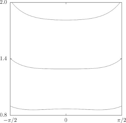
For ω > ωc the top can stand vertically; for ω < ωc the top falls if slightly displaced from the vertical. A top that stands vertically is called a “sleeping” top. For a more realistic top, friction gradually slows the rotation; the rotation rate eventually falls below the critical rotation rate and the top “wakes up.”
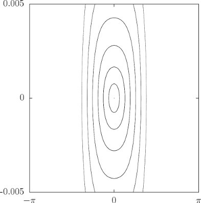
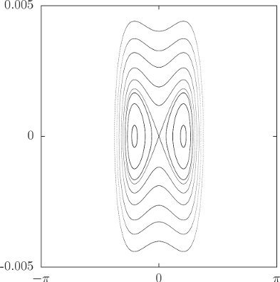
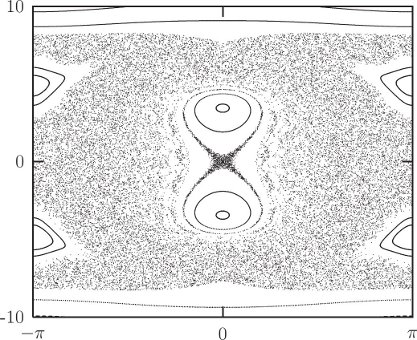
We get additional insight into the sleeping top and the awake top by looking at the trajectories in the θ, pθ phase plane. The trajectories in this plane are simply contours of the Hamiltonian, because the Hamiltonian is conserved. Figure 3.6 shows a phase portrait for ω > ωc. All of the trajectories are loops around the vertical (θ = 0). Displacing the top slightly from the vertical simply places the top on a nearby loop, so the top stays nearly vertical. Figure 3.7 shows the phase portrait for ω < ωc. Here the vertical position is an unstable equilibrium. The trajectories that approach the vertical are asymptotic—they take an infinite amount of time to reach it, just as a pendulum with just the right initial conditions can approach the vertical but never reach it. If the top is displaced slightly from the vertical then the trajectories loop around another center with nonzero θ. A top started at the center point of the loop stays there, and one started near this equilibrium point loops stably around it. Thus we see that when the top “wakes up” the vertical is unstable, but the top does not fall to the ground. Rather, it oscillates around a new equilibrium.
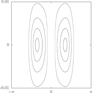
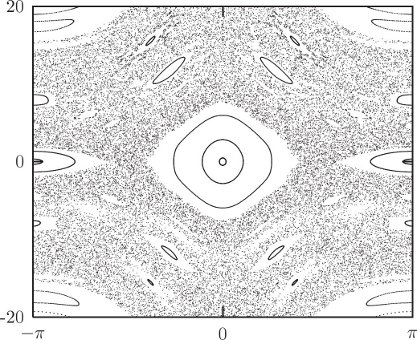
It is also interesting to consider the axisymmetric top when pφ = pψ. Consider the case pφ ≠ pψ. Some trajectories in the θ, pθ plane are shown in figure 3.8. Note that in this case trajectories do not go through θ = 0. The phase portrait for pφ < pψ is similar and is not shown.
We have reduced the motion of the axisymmetric top to quadratures by choosing coordinates that express the symmetries. It turns out that the resulting integrals can be expressed in terms of elliptic functions. Thus, the axisymmetric top can be solved analytically. We do not dwell on this solution because it is not very illuminating: since most problems cannot be solved analytically, there is little profit in dwelling on the analytic solution of one of the rare problems that is analytically solvable. Rather, we have focused on the geometry of the solutions in the phase space and the use of conserved quantities to reduce the dimension of the problem. With the phase-space portrait we have found some interesting qualitative features of the motion of the top.
Exercise 3.8: Sleeping top
Verify that the critical angular velocity above which an axisymmetric top can sleep is given by equation (3.105).
3.4.1 Lagrangian Reduction
Suppose there are cyclic coordinates. In the Hamiltonian formulation, the equations of motion for the coordinates and momenta for the other degrees of freedom form a self-contained subsystem in which the momenta conjugate to the cyclic coordinates are parameters. We can form a Lagrangian for this subsystem by performing a Legendre transform of the reduced Hamiltonian. Alternatively, we can start with the full Lagrangian and perform a Legendre transform for only those coordinates that are cyclic. The equations of motion are Hamilton's equations for those variables that are transformed and Lagrange's equations for the others. The momenta conjugate to the cyclic coordinates are conserved and can be treated as parameters in the Lagrangian for the remaining coordinates.
Divide the tuple q of coordinates into two subtuples q = (x, y). Assume L(t; x, y; vx, vy) is a Lagrangian for the system. Define the Routhian R as the Legendre transform of L with respect to the vy slot:
To define the function R we must solve equation (3.106) for vy in terms of the other variables, and substitute this into equation (3.107).
Define the state path Ξ:
where
Realizable paths satisfy the equations of motion (see exercise 3.9)
which are Lagrange's equations for x and Hamilton's equations for y and py.
Now suppose that the Lagrangian is cyclic in y. Then ∂1,1L = ∂1,1R = 0, and py(t) is a constant c on any realizable path. Equation (3.114) does not depend on y, by assumption, and we can replace py by its constant value c. So equation (3.114) forms a closed subsystem for the path x. The Lagrangian Lc
describes the motion of the subsystem (the minus sign is introduced for convenience, and ● indicates that the function's value is independent of this argument). The path y can be found by integrating equation (3.115) using the independently determined path x.
Define the action
The realizable paths x satisfy the Lagrange equations with the Lagrangian Lc, so the action
For realizable paths q the action S[q](t1, t2) is stationary with respect to variations η of q that are zero at the end times. Along these paths the momentum py(t) has the constant value c. For these same paths the action
The values of the actions
Exercise 3.9: Routhian equations of motion
Verify that the equations of motion are given by equations (3.114–3.116).
3.5 Phase Space Evolution
Most problems do not have enough symmetries to be reducible to quadrature. It is natural to turn to numerical integration to learn more about the evolution of such systems. The evolution in phase space may be found by numerical integration of Hamilton's equations.
As an illustration, consider again the periodically driven pendulum (see page 74). The Hamiltonian is
(show-expression
  ((Lagrangian->Hamiltonian
     (L-periodically-driven-pendulum 'm 'l 'g 'a 'omega))
   (up 't 'theta 'p_theta)))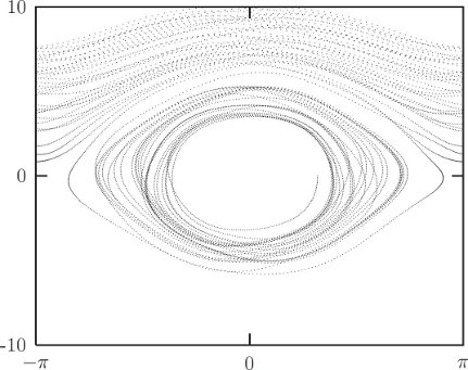
Hamilton's equations for the periodically driven pendulum are un-revealing, so we will not show them. We build a system derivative from the Hamiltonian:
(define (H-pend-sysder m l g a omega)
  (Hamiltonian->state-derivative
    (Lagrangian->Hamiltonian
      (L-periodically-driven-pendulum m l g a omega))))
Now we integrate this system, with the same initial conditions as in section 1.7 (see figure 1.7), but display the trajectory in phase space (figure 3.9), using a monitor procedure:
(define window (frame :-pi :pi -10.0 10.0))

(define ((monitor-p-theta win) state)
  (let ((q ((principal-value :pi) (coordinate state)))
        (p (momentum state)))
    (plot-point win q p)))
We use evolve to explore the evolution of the system:
(let ((m 1.0)           ;m=1 kg
      (l 1.0)           ;l=1 m
      (g 9.8)           ;g=9.8 m/s²
      (A 0.1)           ;A=1/10 m
      (omega (* 2 (sqrt 9.8)))
      ((evolve H-pend-sysder m l g A omega)
       (up 0.0          ;t₀=0
           1.0          ;θ₀=1 rad
           0.0)         ;p₀=0 kg m²/s
       (monitor-p-theta window)
       0.01             ;plot interval
       100.0            ;final time
       1.0e-12)))
The trajectory sometimes oscillates and sometimes circulates. The patterns in the phase plane are reminiscent of the trajectories in the phase plane of the undriven pendulum shown in figure 3.4 on page 225.
3.5.1 Phase-Space Description Is Not Unique
We are familiar with the fact that a given motion of a system is expressed differently in different coordinate systems: the functions that express a motion in rectangular coordinates are different from the functions that express the same motion in polar coordinates. However, in a given coordinate system the evolution of the local state tuple for particular initial conditions is unique. The generalized velocity path function is the derivative of the generalized coordinate path function. On the other hand, the coordinate system alone does not uniquely specify the phase-space description. The relationship of the momentum to the coordinates and the velocities depends on the Lagrangian, and many different Lagrangians may be used to describe the behavior of the same physical system. When two Lagrangians for the same physical system are different, the phase-space descriptions of a dynamical state are different.
We have already seen two different Lagrangians for the driven pendulum (see section 1.6.4): one was found using L = T −V and the other was found by inspection of the equations of motion. The two Lagrangians differ by a total time derivative. The momentum pθ conjugate to θ depends on which Lagrangian we choose to work with, and the description of the evolution in the corresponding phase space also depends on the choice of Lagrangian, even though the behavior of the system is independent of the method used to describe it. The momentum conjugate to θ, using the L = T − V Lagrangian for the periodically driven pendulum, is
but with the alternative Lagrangian, it is
The two momenta differ by an additive distortion that varies periodically in time and depends on θ. That the phase-space descriptions are different is illustrated in figure 3.10. The evolution of the system is the same for each.
3.6 Surfaces of Section
Computing the evolution of mechanical systems is just the beginning of understanding the dynamics. Typically, we want to know much more than the phase space evolution of some particular trajectory. We want to obtain a qualitative understanding of the motion. We want to know what sorts of motion are possible, and how one type relates to others. We want to abstract the essential dynamics from the myriad particular evolutions that we can calculate. Paradoxically, it turns out that by throwing away most of the calculated information about a trajectory we gain essential new information about the character of the trajectory and its relation to other trajectories.
A remarkable tool that extracts the essence by throwing away information is a technique called the surface of section or Poincaré section.23 A surface of section is generated by looking at successive intersections of a trajectory or a set of trajectories with a plane in the phase space. Typically, the plane is spanned by a coordinate axis and the canonically conjugate momentum axis. We will see that surfaces of section made in this way have nice properties.
The surface of section technique was put to spectacular use in the 1964 landmark paper [22] by astronomers Michel Hénon and Carl Heiles. In their numerical investigations they found that some trajectories are chaotic, whereas other trajectories are regular. An essential characteristic of the chaotic motions is that initially nearby trajectories separate exponentially with time; the separation of regular trajectories is linear.24 They found that these two types of trajectories are typically clustered in the phase space into regions of regular motion and regions of chaotic motion.
3.6.1 Periodically Driven Systems
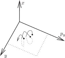
For a periodically driven system the surface of section is a stroboscopic view of the evolution; we consider only the state of the system at the strobe times, with the period of the strobe equal to the drive period. We generate a surface of section for a periodically driven system by computing a number of trajectories and accumulating the phase-space coordinates of each trajectory whenever the drive passes through some particular phase. Let T be the period of the drive; then, for each trajectory, the surface of section accumulates the phase-space points (q(t), p(t)), (q(t + T), p(t + T)), (q(t + 2T), p(t + 2T)), and so on (see figure 3.11). For a system with a single degree of freedom we can plot the sequence of phase-space points on a q, p surface.
In the case of the stroboscopic section for the periodically driven system, the phase of the drive is the same for all section points; thus each phase-space point in the section, with the known phase of the drive, may be considered as an initial condition for the rest of the trajectory. The absolute time of the particular section point does not affect the subsequent evolution; all that matters is that the phase of the drive have the value specified for the section. Thus we can think of the dynamical evolution as generating a map that takes a point in the phase space and generates a new point in the phase space after evolving the system for one drive period. This map of the phase space onto itself is called the Poincaré map.
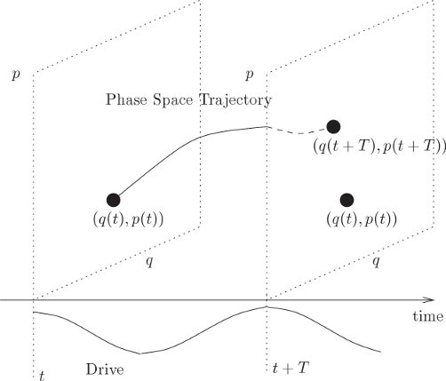
Figure 3.12 shows an example Poincaré section for the driven pendulum. We plot the section points for a number of different initial conditions. We are immediately presented with a new facet of dynamical systems. For some initial conditions, the subsequent section points appear to fill out a set of curves in the section. For other initial conditions this is not the case: rather, the set of section points appear scattered over a region of the section. In fact, all of the scattered points in figure 3.12 were generated from a single initial condition. The surface of section suggests that there are qualitatively different classes of trajectories distinguished by the dimension of the subspace of the section that they explore.
Trajectories that fill out curves on the surface of section are called regular or quasiperiodic trajectories. The curves that are filled out by the regular trajectories are invariant curves. They are invariant in that if any section point for a trajectory falls on an invariant curve, all subsequent points fall on the same invariant curve. Otherwise stated, the Poincaré map maps every point on an invariant curve onto the invariant curve.
The trajectories that appear to fill areas are called chaotic trajectories. For these points the distance in phase space between initially nearby points grows, on average, exponentially with time.25 In contrast, for the regular trajectories, the distance in phase space between initially nearby points grows, on average, linearly with time.
The phase space seems to be grossly clumped into different regions. Initial conditions in some regions appear to predominantly yield regular trajectories, and other regions appear to predominantly yield chaotic trajectories. This gross division of the phase space into qualitatively different types of trajectories is called the divided phase space. We will see later that there is much more structure here than is apparent at this scale, and that upon magnification there is a complicated interweaving of chaotic and regular regions on finer and finer scales. Indeed, we shall see that many trajectories that appear to generate curves on the surface of section are, upon magnification, actually chaotic and fill a tiny area. We shall also find that there are trajectories that lie on one-dimensional curves on the surface of section, but only explore a subset of this curve formed by cutting out an infinite number of holes.26
The features seen on the surface of section of the driven pendulum are quite general. The same phenomena are seen in most dynamical systems. In general, there are both regular and chaotic trajectories, and there is the clumping characteristic of the divided phase space. The specific details depend upon the system, but the basic phenomena are generic. Of course, we are interested in both aspects: the phenomena that are common to all systems, and the specific details for particular systems of interest.
The surface of section for the periodically driven pendulum has specific features that give us qualitative information about how this system behaves. The central island in figure 3.12 is the remnant of the oscillation region for the unforced pendulum (see figure 3.4 in section 3.3). There is a sizable region of regular trajectories here that are, in a sense, similar to the trajectories of the unforced pendulum. In this region, the pendulum oscillates back and forth, much as the undriven pendulum does, but the drive makes it wiggle as it does so. The section points are all collected at the same phase of the drive so we do not see these wiggles on the section.
The central island is surrounded by a large chaotic zone. Thus the region of phase space with regular trajectories similar to the unforced trajectories has finite extent. On the section, the boundary of this “stable” region is apparently rather well defined—there is a sudden transition from smooth regular invariant curves to chaotic motion that can take the system far from this region of regular motion.
There are two other sizeable regions of regular behavior with finite angular extent. The trajectories in these regions are resonant with the drive, on average executing one full rotation per cycle of the drive. The two islands differ in the direction of the rotation. In these regions the pendulum is making complete rotations, but the rotation is locked to the drive so that points on the section appear only in the islands. The fact that points for particular trajectories loop around the islands means that the pendulum sometimes completes a cycle faster than the drive and sometimes slower than the drive, but never loses lock.
Each regular region has finite extent. So from the surface of section we can see directly the range of initial conditions that remain in resonance with the drive. Outside of the regular region initial conditions lead to chaotic trajectories that evolve far from the resonant regions.
Various higher-order resonance islands are also visible, as are nonresonant regular circulating orbits. So, the surface of section has provided us with an overview of the main types of motion that are possible and their interrelationship.
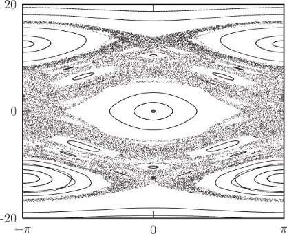
Changing the parameters shows other interesting phenomena. Figure 3.13 shows the surface of section when the drive frequency is twice the natural small-amplitude oscillation frequency of the undriven pendulum. The section has a large chaotic zone, with an interesting set of islands. The central equilibrium has undergone an instability and instead of a central island we find two off-center islands. These islands are alternately visited one after the other. As the support goes up and down the pendulum alternately tips to one side and then the other. It takes two periods of the drive before the pendulum visits the same island. Thus, the system has “period-doubled.” An island has been replaced by a period-doubled pair of islands. Note that other islands still exist. The islands in the top and bottom of the chaotic zone are the resonant islands, in which the pendulum loops on average a full turn for every cycle of the drive. Note that, as before, if the pendulum is rapidly circulating, the motion is regular.
It is a surprising fact that if we shake the support of a pendulum fast enough then the pendulum can stand upright. This phenomenon can be visualized with the surface of section. Figure 3.14 shows a surface of section when the drive frequency is large compared to the natural frequency. That the pendulum can stand upright is indicated by the existence of a regular island at the inverted equilibrium. The surface of section shows that the pendulum can remain upright for a range of initial displacements from the vertical.
3.6.2 Computing Stroboscopic Surfaces of Section
We already have the system derivative for the driven pendulum, and we can use it to make a parametric map for constructing Poincaré sections:
(define (driven-pendulum-map m l g A omega)
  (let ((advance (state-advancer H-pend-sysder m l g A omega))
        (map-period (/ :2pi omega)))
    (lambda (theta ptheta return fail)
      (let ((ns (advance
                  (up 0 theta ptheta) ; initial state</span></td>
                  map-period))) ; integration interval</span></td>
        (return ((principal-value :pi)
                 (coordinate ns))
                (momentum ns))))))
A map procedure takes the two section coordinates (here theta and ptheta) and two “continuation” procedures. If the section coordinates given are in the domain of the map, it produces two new section coordinates and passes them to the return continuation, otherwise the map procedure calls the fail continuation procedure with no arguments.27
The trajectories of a map can be explored with an interactive interface. The procedure explore-map lets us use a pointing device to choose initial conditions for trajectories. For example, the surface of section in figure 3.12 was generated by plotting a number of trajectories, using a pointer to choose initial conditions, with the following program:
(define win (frame :-pi :pi -20 20))
(let ((m 1.0)   ;m=1kg
      (l 1.0)   ;l=1m
      (g 9.8)   ;g=9.8m/s^2
      (A 0.05)) ;A=1/20m
  (let ((omega0 (sqrt (/ g l))))
    (let ((omega (* 4.2 omega0)))
      (explore-map
        win
        (driven-pendulum-map m l g A omega)
        1000)))) ;1000 points for each initial condition
Exercise 3.10: Fun with phase portraits
Choose some one-degree-of-freedom dynamical system that you are curious about and that can be driven with a periodic drive. Construct a map of the sort we made for the driven pendulum and do some exploring. Are there chaotic regions? Are all of the chaotic regions connected together?
3.6.3 Autonomous Systems
We illustrated the use of Poincaré sections to visualize qualitative features of the phase space for a one-degree-of-freedom system with periodic drive, but the idea is more general. Here we show how Hénon and Heiles [22] used the surface of section to elucidate the properties of an autonomous system.
Hénon–Heiles background
In the early '60s astronomers were up against a wall. Careful measurements of the motion of nearby stars in the galaxy had allowed particular statistical averages of the observed motions to be determined, and the averages were not at all what was expected. In particular, what was calculated was the velocity dispersion: the root mean square deviation of the velocity from the average. We use angle brackets to denote an average over nearby stars: < w > is the average value of some quantity w for the stars in the ensemble. The average velocity is
If we use cylindrical polar coordinates (r, θ, z) and align the axes with the galaxy so that z is perpendicular to the galactic plane and r increases with the distance to the center of the galaxy, then two particular components of the velocity dispersion are
It was expected at the time that these two components of the velocity dispersion should be equal. In fact they were found to differ by about a factor of 2: σr ≈ 2σz. What was the problem? In the literature at the time there was considerable discussion of what could be wrong. Was the problem some observational selection effect? Were the velocities measured incorrectly? Were the assumptions used in the derivation of the expected ratio not adequately satisfied? For example, the derivation assumed that the galaxy was approximately axisymmetric. Perhaps non-axisymmetric components of the galactic potential were at fault. It turned out that the problem was much deeper. The understanding of motion was wrong.
Let's review the derivation of the expected relation among the components of the velocity dispersion. We wish to give a statistical description of the distribution of stars in the galaxy. We introduce the phase-space distribution function
where the integral extends over the phase-space volume V. In computing the velocity dispersion at some point
Individual stars move in the gravitational potential of the rest of the galaxy. It is not unreasonable to assume that the overall distribution of stars in the galaxy does not change much with time, or changes only very slowly. The density of stars in the galaxy is actually very small and close encounters of stars are very rare. Thus, we can model the gravitational potential of the galaxy as a fixed external potential in which individual stars move. The galaxy is approximately axisymmetric. We assume that the deviation from exact axisymmetry is not a significant effect and thus we take the model potential to be exactly axisymmetric.
Consider the motion of a point mass (a star) in an axisymmetric potential (of the galaxy). In cylindrical polar coordinates the Hamiltonian is
where V does not depend on θ. Since θ does not appear, we know that the conjugate momentum pθ is constant. For the motion of any particular star we can treat pθ as a parameter. Thus the effective Hamiltonian has two degrees of freedom:
where
The value E of the Hamiltonian is constant since there is no explicit time dependence in the Hamiltonian. Thus, we have constants of the motion E and pθ.
Jeans's “theorem” asserts that the distribution function f depends only on the values of the conserved quantities, also known as integrals of motion. That is, we can introduce a different distribution function f′ that represents the same physical distribution:
At the time, there was good reason to believe that this might be correct. First, it is clear that the distribution function surely depends at least on E and pθ. The problem is, “Given an energy E and angular momentum pθ, what motion is allowed?” The conserved quantities clearly confine the evolution. Does the evolution carry the system everywhere in the phase space subject to these known constraints? In the early part of the 20th century this appeared plausible. Statistical mechanics was successful, and statistical mechanics made exactly this assumption. Perhaps there are other conserved quantities of the motion that exist, but that we have not yet discovered?
Poincaré proved an important theorem with regard to conserved quantities. Poincaré proved that most of the conserved quantities of a dynamical system typically do not persist upon perturbation of the system. That is, if a small perturbation is added to a problem, then most of the conserved quantities of the original problem do not have analogs in the perturbed problem. The conserved quantities are destroyed. However, conserved quantities that result from symmetries of the problem continue to be preserved if the perturbed system has the same symmetries. Thus angular momentum continues to be preserved upon application of any axisymmetric perturbation. Poincaré's theorem is correct, but what came next was not.
As a corollary to Poincaré's theorem, in 1920 Fermi published a proof of a theorem stating that typically the motion of perturbed problems is ergodic29 subject to the constraints imposed by the conserved quantities resulting from symmetries. Loosely speaking, this means that trajectories go everywhere they are allowed to go by the conservation constraints. Fermi's theorem was later shown to be incorrect, but on the basis of this theorem we could expect that typically systems fully explore the phase space, subject only to the constraints imposed by the conserved quantities resulting from symmetries. Suppose then that the evolution of stars in the galactic potential is subject only to the constraints of conserving E and pθ. We shall see that this is not true, but if it were we could then conclude that the distribution function for stars in the galaxy can also depend only on E and pθ.
Given this form of the distribution function, we can deduce the stated ratios of the velocity dispersions. We note that pz and pr appear in the same way in the energy. Thus the average of any function of pz computed with the distribution function must equal the average of the same function of pr. In particular, the velocity dispersions in the z and r directions must be equal:
But this is not what was observed, which was
Hénon and Heiles [22] approached this problem differently from others at the time. Rather than improving the models for the motion of stars in the galaxy, they concentrated on what turned out to be the central issue: What is the qualitative nature of motion? The problem had nothing to do with galactic dynamics in particular, but with the problem of motion. They abstracted the dynamical problem from the particulars of galactic dynamics.
The system of Hénon and Heiles
We have seen that the study of the motion of a point with mass m and an axisymmetric potential energy reduces to the study of a reduced two-degree-of-freedom problem in r and z with potential energy U(r, z). Hénon and Heiles chose to study the motion in a two-degree-of-freedom system with a particularly simple potential energy so that the dynamics would be clear and the calculation uncluttered. The Hénon–Heiles Hamiltonian is
with potential energy
The potential energy is shaped like a distorted bowl. It has triangular symmetry, as is evident when it is rewritten in polar coordinates:
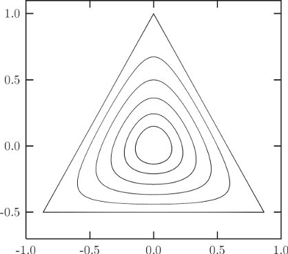
Contours of the potential energy are shown in figure 3.15. At small values of the potential energy the contours are approximately circular; as the value of the potential energy approaches 1/6 the contours become triangular, and at larger potential energies the contours open to infinity.
The Hamiltonian is independent of time, so energy is conserved. In this case this is the only known conserved quantity. We first determine the restrictions that conservation of energy imposes on the evolution. We have
so the motion is confined to the region inside the contour V = E because the sum of the squares of the momenta cannot be negative.
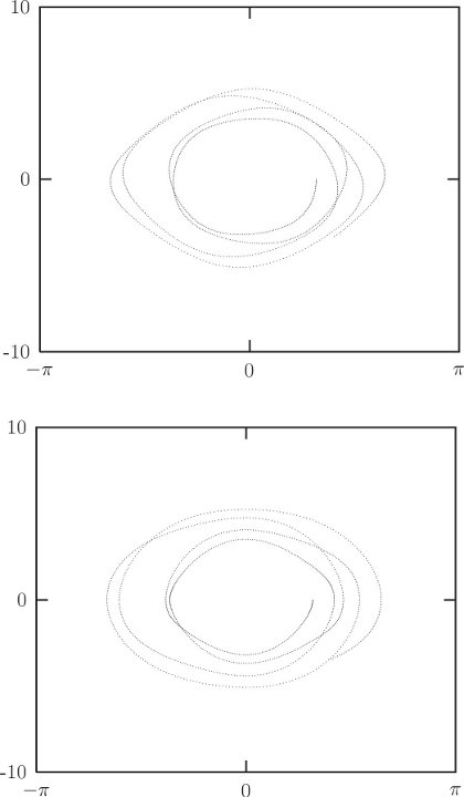
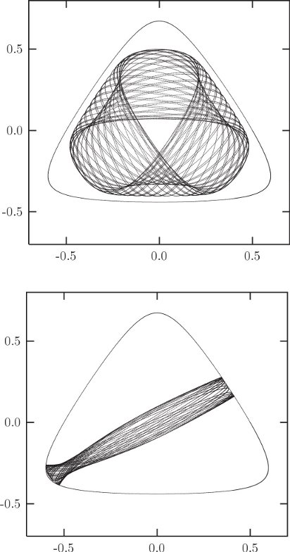
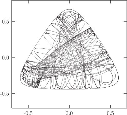
Let's compute some sample trajectories. For definiteness, we investigate trajectories with energy E = 1/8. There is a large variety of trajectories. There are trajectories that circulate in a regular way around the bowl, and there are trajectories that oscillate back and forth (figure 3.16). There are also trajectories that appear more irregular (figure 3.17). There is no end to the trajectories that could be computed, but let's face it, surely there is more to life than looking at trajectories.
The problem facing Hénon and Heiles was the issue of conserved quantities. Are there other conserved quantities besides the obvious ones? They investigated this issue with the surface of section technique. The surface of section is generated by looking at successive passages of trajectories through a plane in phase space.
Specifically, the surface of section is generated by recording and plotting py versus y whenever x = 0, as shown in figure 3.18. Given the value of the energy E and a point (y, py) on the section x = 0, we can recover px, up to a sign. If we restrict attention to intersections with the section plane that cross with, say, positive px, then there is a one-to-one relation between section points and trajectories. A section point thus corresponds to a unique trajectory.
How does this address the issue of the number of conserved quantities? A priori, there appear to be two possibilities: either there are hidden conserved quantities or there are not. Suppose there is no other conserved quantity besides the energy. Then the expectation was that successive intersections of the trajectory with the section plane would eventually explore all of the section plane that is consistent with conservation of energy. On the other hand, if there is a hidden conserved quantity then the successive intersections would be constrained to fall on a curve.
Interpretation
On the section, the energy is
Because
So, if there is no other conserved quantity, we might expect the points on the section eventually to fill the area enclosed by this bounding curve.
On the other hand, suppose there is a hidden extra conserved quantity I(x, y; px, py) = 0. Then this conserved quantity would provide further constraints on the trajectories and their intersections with the section plane. An extra conserved quantity I provides a constraint among the four phase-space variables x, y, px, and py. We can use E to solve for px, so for a given E, I gives a relation among x, y, and py. Using the fact that on the section x = 0, the I gives a relation between y and py on the section for a given E. So we expect that if there is another conserved quantity the successive intersections of a trajectory with the section plane will fall on a curve.
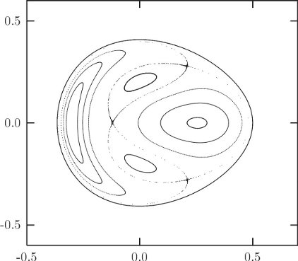
If there is no extra conserved quantity we expect the section points to fill an area; if there is an extra conserved quantity we expect the section points to be restricted to a curve. What actually happens? Figure 3.19 shows a surface of section for E = 1/12; the section points for several representative trajectories are displayed. By and large, the points appear to be restricted to curves, so there appears to be evidence for an extra conserved quantity. Look closely though. Where the “curves” cross, the lines are a little fuzzy. Hmmm.
Let's try a little larger energy, E = 1/8. The appearance of the section changes qualitatively (figure 3.20). For some trajectories there still appear to be extra constraints on the motion. But other trajectories appear to fill an area of the section plane, pretty much as we expected of trajectories if there was no extra conserved quantity. In particular, all of the scattered points on this section were generated by a single trajectory. Thus, some trajectories behave as if there is an extra conserved quantity, and others don't. Wow!
Let's go on to a higher energy, E = 1/6, just at the escape energy. A section for this energy is shown in figure 3.21. Now, a single trajectory explores most of the region of the section plane allowed by energy conservation, but not entirely. There are still trajectories that appear to be subject to extra constraints.
We seem to have all possible worlds. At low energy, the system by and large behaves as if there is an extra conserved quantity, but not entirely. At intermediate energy, the phase space is divided: some trajectories explore areas whereas others are constrained. At high energy, trajectories explore most of the energy surface; few trajectories show extra constraints. We have just witnessed our first transition to chaos.
Two qualitatively different types of motion are revealed by this surface of section, just as we saw in the Poincaré sections for the driven pendulum. There are trajectories that seem to be constrained as if by an extra conserved quantity. And there are trajectories that explore an area on the section as though there were no extra conserved quantitiess. Regular trajectories appear to be constrained by an extra conserved quantity to a one-dimensional set on the section; chaotic trajectories are not constrained in this way and explore an area.30
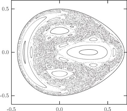
The surface of section not only reveals the existence of qualitatively different types of motion, but also provides an overview of the different types of trajectories. Take the surface of section for E = 1/8 (figure 3.20). There are four main islands, engulfed in a chaotic sea. The particular trajectories displayed above provide examples from different parts of the section. The trajectory that loops around the bowl (figure 3.16) belongs to the large island on the left side of the section. Similar trajectories that loop around the bowl in the other direction belong to the large island on the right side of the section. The trajectories that oscillate back and forth across the bowl belong to the two islands above and below the center of the section. (By symmetry there should be three such islands. The third island is snugly wrapped against the boundary of the section.) Each of the main islands is surrounded by a chain of secondary islands. We will see that the types of orbits are inexhaustible, if we look closely enough. The chaotic trajectory (figure 3.17) lives in the chaotic sea. Thus the section provides a summary of the types of motion possible and how they are related to one another. It is much more useful than plots of a zillion trajectories.
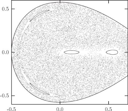
The section for a particular energy summarizes the dynamics at that energy. A sequence of sections for various energies shows how the major features change with the energy. We have already noticed that at low energy the section is dominated by regular orbits, at intermediate energy the section is divided more or less equally into regular and chaotic regions, and at high energies the section is dominated by a single chaotic zone. We will see that such transitions from regular to chaotic behavior are quite common; similar phenomena occur in widely different systems, though the details depend on the system under study.
3.6.4 Computing Hénon–Heiles Surfaces of Section
The following procedures implement the Poincaré map for the Hénon–Heiles system:
(define (HHmap E dt sec-eps int-eps)
  (define ((make-advance advancer eps) s dt)
    (advancer s dt eps))
  (let ((adv
          (make-advance (state-advancer HHsysder) int-eps)))
    (lambda (y py cont fail)
      (let ((initial-state (section->state E y py)))
        (if (not initial-state)
          (fail)
          (find-next-crossing initial-state adv dt sec-eps
                              (lambda (crossing-state running-state)
                                (cont (ref (coordinate crossing-state)
                                           1)
                                      (ref (momentum crossing-state)
                                           1)))))))))
Besides supplying the energy E of the section we must also supply a time step for the integrator to achieve, a tolerance for a point to be on the section sec-eps, and a local truncation error specification for the integrator int-eps.
For each initial point (y, py) on the surface of section, the map first finds the initial state that has the specified energy, if one exists. The procedure section->state handles this task:
(define (section->state E y py)
  (let ((d (- E (+ (HHpotential (up 0 (up 0 y)))
                   (* 1/2 (square py))))))
    (if (>= d 0.0)
      (let ((px (sqrt (* 2 d))))
        (up 0 (up 0 y) (down px py)))
      #f)))
The procedure section->state returns #f (false) if there is no state consistent with the specified energy.
The Hamiltonian procedure for the Hénon–Heiles problem is
(define (HHHam s)
  (+ (* 1/2 (square (momentum s)))
     (HHpotential s)))
with the potential energy
(define (HHpotential s)
  (let ((x (ref (coordinate s) 0))
        (y (ref (coordinate s) 1)))
    (+ (* 1/2 (+ (square x) (square y)))
       (- (* (square x) y) (* 1/3 (cube y))))))
The system derivative is computed directly from the Hamiltonian.
(define (HHsysder)
  (Hamiltonian->state-derivative HHHam))
The procedure find-next-crossing advances the initial state until successive states are on opposite sides of the section plane.
(define (find-next-crossing state advance dt sec-eps cont)
  (let lp ((s state))
    (let ((next-state (advance s dt)))
      (if (and (> (ref (coordinate next-state) 0) 0)
               (< (ref (coordinate s) 0) 0))
        (let ((crossing-state
                (refine-crossing sec-eps advance s)))
          (cont crossing-state next-state))
        (lp next-state)))))
After finding states that straddle the section plane the crossing is refined by Newton's method, as implemented by the procedure refine-crossing. The procedure find-next-crossing returns both the crossing point and the next state produced by the integrator. The next state is not used in this problem but it is needed for other cases.
(define (refine-crossing sec-eps advance state)
  (let lp ((state state))
    (let ((x (ref (coordinate state) 0))
          (xd (ref (momentum state) 0)))
      (let ((zstate (advance state (- (/ x xd)))))
        (if (< (abs (ref (coordinate zstate) 0))
               sec-eps)
          zstate
          (lp zstate))))))
To explore the Hénon–Heiles map we use explore-map as before. The following exploration generated figure 3.20:
(define win (frame -0.5 0.7 -0.6 0.6))
(explore-map win (HHmap 0.125 0.1 1.0e-10 1.0e-12) 500)
3.6.5 Non-Axisymmetric Top
We have seen that the motion of an axisymmetric top can be essentially solved. A plot of the rate of change of the tilt angle versus the tilt angle is a simple closed curve. The evolution of the other angles describing the configuration can be obtained by quadrature once the tilting motion has been solved. Now let's consider a non-axisymmetric top. A non-axisymmetric top is a top with three unequal moments of inertia. The pivot is not at the center of mass, so uniform gravity exerts a torque. We assume the line between the pivot and the center of mass is one of the principal axes, which we take to be ĉ. There are no torques about the vertical axis, so the vertical component of the angular momentum is conserved. If we write the Hamiltonian in terms of the Euler angles, the angle φ, which corresponds to rotation about the vertical, does not appear. Thus the momentum conjugate to this angle is conserved. The nontrivial degrees of freedom are θ and ψ, with their conjugate momenta.
We can make a surface of section (see figure 3.22) for this problem by displaying pθ versus θ when ψ = 0. There are in general two values of pψ possible for given values of energy and pφ. We plot points only if the value of pψ at the crossing is the larger of the two possibilities. This makes the points of the section correspond uniquely to a trajectory.
In this section there is a large quasiperiodic island surrounding a fixed point that corresponds to the tilted equilibrium point of the awake axisymmetric top (see figure 3.7 in section 3.4). Surrounding this is a large chaotic zone that extends from θ = 0 to angles near π. If this top is placed initially near the vertical, it exhibits chaotic motion that carries it to large tilt angles. If the top is started within the quasiperiodic island, the tilt is stable.
3.7 Exponential Divergence
Hénon and Heiles discovered that the chaotic trajectories had remarkable sensitivity to small changes in initial conditions—initially nearby chaotic trajectories separate roughly exponentially with time. On the other hand, regular trajectories do not exhibit this sensitivity—initially nearby regular trajectories separate roughly linearly with time.
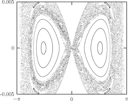
Consider the evolution of two initially nearby trajectories for the Hénon–Heiles problem, with energy E = 1/8. Let d(t) be the usual Euclidean distance in the x, y, px, py space between the two trajectories at time t. Figure 3.23 shows the common logarithm of d(t)/d(0) as a function of time t. We see that the divergence is well described as exponential.
On the other hand, the distance between two initially nearby regular trajectories grows much more slowly. Figure 3.24 shows the distance between two regular trajectories as a function of time. The distance grows linearly with time.
It is remarkable that Hamiltonian systems have such radically different types of trajectories. On the surface of section the chaotic and regular trajectories differ in the dimension of the space that they explore. It is interesting that along with this dimensional difference there is a drastic difference in the way chaotic and regular trajectories separate. For higher-dimensional systems the surface of section technique is not as useful, but trajectories are still distinguished by the way neighboring trajectories diverge: some diverge exponentially whereas others diverge approximately linearly. Exponential divergence is the hallmark of chaotic behavior.
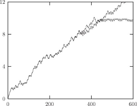
The rate of exponential divergence is quantified by the slope of the graph of log(d(t)/d(0)). We can estimate the rate of exponential divergence of trajectories from a particular phase-space trajectory σ by choosing a nearby trajectory σ′ and computing
where d(t) = ‖σ′ (t)−σ(t)‖. A problem with this “two-trajectory” method is illustrated in figure 3.23. For strongly chaotic trajectories two initially nearby trajectories soon find themselves as far apart as they can get. Once this happens the distance no longer grows. The estimate of the rate of divergence of trajectories is limited by this saturation.
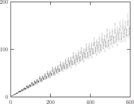
We can improve on this method by studying a variational system of equations. Let
be the system of equations governing the evolution of the system. A nearby trajectory z′ satisfies
The difference ζ = z′ − z between these trajectories satisfies
If ζ is small we can approximate the right-hand side by a derivative
This set of ordinary differential equations is called the variational equations for the system. It is linear in ζ and driven by z.
Let d(t) = ‖ζ(t)‖; then the rate of divergence can be estimated as before. The advantage of this “variational method” is that ζ(t) can become arbitrarily large and its growth still measures the divergence of nearby trajectories. We can see in figure 3.23 that the variational method gives nearly the same result as the two-trajectory method up to the point at which the two-trajectory method saturates.31
The Lyapunov exponent is defined to be the infinite time limit of γ(t), defined by equation (3.141), in which the distance d is computed by the variational method. Actually, for each trajectory there are many Lyapunov exponents, depending on the initial direction of the variation ζ. For an N-dimensional system, there are N Lyapunov exponents. For a randomly chosen ζ(t0), the subsequent growth of ζ(t) has components that grow with each of the Lyapunov exponents. In general, however, the growth of ζ(t) will be dominated by the largest exponent. The largest Lyapunov exponent thus can be interpreted as the typical rate of exponential divergence of nearby trajectories. The sum of the largest two Lyapunov exponents can be interpreted as the typical rate of growth of the area of two-dimensional elements. This interpretation can be extended to higher-dimensional elements: the rate of growth of volume elements is the sum of all the Lyapunov exponents.
In Hamiltonian systems, the Lyapunov exponents must satisfy the following constraints. Lyapunov exponents come in pairs; for every Lyapunov exponent λ, its negation −λ is also an exponent. For every conserved quantity, one of the Lyapunov exponents is zero, as is its negation. So the Lyapunov exponents can be used to check for the existence of conserved quantities. The sum of the Lyapunov exponents for a Hamiltonian system is zero, so volume elements do not grow exponentially. We will see in the next section that phase-space volume is actually conserved for Hamiltonian systems.
3.8 Liouville's Theorem
If an ensemble of states occupies a particular volume of phase space at one moment, then the subsequent evolution of that volume by the flow described by Hamilton's equations may distort the ensemble but does not change the volume the ensemble occupies. The fact that phase-space volume is preserved by the phase flow is called Liouville's theorem.
We will first illustrate the preservation of phase-space volume with a simple example and then prove it in general.
The phase flow for the pendulum
Consider an undriven pendulum described by the Hamiltonian
In figure 3.25 we see the evolution of an elliptic region around a point on the θ-axis, in the oscillation region of the pendulum. Three later positions of the region are shown. The region is stretched and sheared by the flow, but the area is preserved. After many cycles, the starting region will be stretched to be a thin layer distributed in the phase angle of the pendulum. Figure 3.26 shows a similar evolution (for smaller time intervals) of a region straddling the separatrix32 near the unstable equilibrium point. The phase-space region rapidly stretches along the separatrix, while preserving the area. The initial conditions that start in the oscillation region (inside of the separatrix) will continue to spread into a thin ring-shaped region, while the initial conditions that start outside of the separatrix will spread into a thin region of rotation on the outside of the separatrix.
Proof of Liouville's theorem
Consider a set of ordinary differential equations of the form
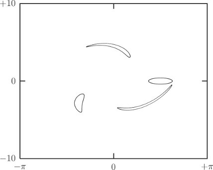
where z is a tuple of N state variables. Let R(t1) be a region of the state space at time t1. Each element of this region is an initial condition at time t1 for the system, and evolves to an element at time t2 according to the differential equations. The set of these elements at time t2 is the region R(t2). Regions evolve to regions.
The evolution of the system for a time interval Δt defines a map gt,Δt from the state space to itself:
Regions map to regions by mapping each element in the region:
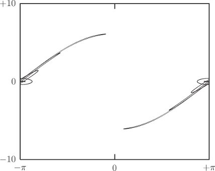
The volume V (t) of a region R(t) is
where Jac(gt,Δt) is the Jacobian of the mapping gt,Δt. The Jacobian is the determinant of the derivative of the mapping.
For small Δt
and thus
where I is the identity function, so DI(z(t)) is a unit multiplier. We can use the fact that if A is an N × N square matrix then
to show that
where
Thus
So the rate of change of the volume at time t is
Now we compute Gt for a system described by a Hamiltonian H. The components of z are the components of the coordinates and the momenta: zk = qk and zk+n = pk for k = 0, …, n − 1. The components of F are
for k = 0, …, n − 1. The diagonal components of the derivative ∂1F are
The component partial derivatives commute, so the diagonal components with index k and index k + n are equal and opposite. We see that the trace, which is the sum of these diagonal components, is zero. Thus the integral of Gt over the region R(t) is zero, so the derivative of the volume at time t is zero. Because t is arbitrary, the volume does not change. This proves Liouville's theorem: the phase-space flow conserves phase-space volume.
Notice that the proof of Liouville's theorem does not depend upon whether or not the Hamiltonian has explicit time dependence. Liouville's theorem holds for systems with time-dependent Hamiltonians.
We may think of the ensemble of all possible states as a fluid flowing around under the control of the dynamics. Liouville's theorem says that this fluid is incompressible for Hamiltonian systems.
Exercise 3.11: Determinants and traces
Show that equation (3.153) is correct.
Area preservation of stroboscopic surfaces of section
Surfaces of section for periodically driven Hamiltonian systems are area preserving if the section coordinates are the phase-space coordinate and momentum. This is an important feature of surfaces of section. It is a consequence of Liouville's theorem for one-degree-of-freedom problems.
It is also the case that surfaces of section such as those we have used for the Hénon–Heiles problem are area preserving, but we are not ready to prove this yet!
Poincaré recurrence
The Poincaré recurrence theorem is a remarkable theorem that is a trivial consequence of Liouville's theorem. Loosely, the theorem states that almost all trajectories eventually return arbitrarily close to where they started. This is true regardless of whether the trajectories are chaotic or regular.
More precisely, consider a Hamiltonian dynamical system for which the phase space is a bounded domain D. We identify some initial point in the phase space, say z0. Then, for any finite neighborhood U of z0 we choose, there are trajectories that emanate from initial points in that neighborhood and eventually return to the neighborhood.
We can prove this by considering the successive images of U under the time evolution. For simplicity, we restrict consideration to time evolution for a time interval Δ. The map of the phase space onto itself generated by time evolution for an interval Δ we call C. Subsequent applications of the map generate a discrete time evolution. Sets of points in phase space transform by evolving all the points in the set; the image of the set U is denoted C(U). Now consider the trajectory of the set U, that is, the sets Cn(U) where Cn indicates the n-times composition of C. Now there are two possibilities: either the successive images Ci(U) intersect or they do not. If they do not intersect, then with each iteration, a volume of D equal to the volume of U gets “used up” and cannot belong to the further image. But the volume of D is finite, so we cannot fit an infinite number of non-intersecting finite volumes into it. Therefore, after some number of iterations the images intersect. Suppose Ci(U) intersects with Cj(U), with j < i, for definiteness. Then the pre-image of each must also intersect, since the pre-image of a point in the intersection belongs to both sets. Thus Ci−1(U) intersects Cj−1(U). This can be continued until finally we have that Ci−j(U) intersects U. So we have proven that after i − j iterations of the map C there are a set of points initially in U that return to the neighborhood U.
So for every neighborhood of every point in the phase space there is a subneighborhood such that the trajectories emanating from all of the points in that subneighborhood return to that subneighborhood. Thus almost every trajectory returns arbitrarily close to where it started.
The gas in the corner of the room
Suppose we have a collection of N classical atoms in a perfectly sealed room. The phase-space dimension of this system is 6N. A point in this phase space is denoted z. Suppose that initially all the atoms are, say, within one centimeter of one corner, with arbitrarily chosen finite velocities. This corresponds to some initial point z0 in the phase space. The phase space of the system is limited in space by the room and in momentum by energy conservation; the phase space is bounded. The recurrence theorem then says that in the neighborhood of z0 there is an initial condition of the system that returns to the neighborhood of z0 after some time. For the individual atoms this means that after some time all of the atoms will be found in the corner of the room again, and again, and again. Makes one wonder about the second law of thermodynamics, doesn't it?33
Nonexistence of attractors in Hamiltonian systems
Some systems have attractors. An attractor is a region of phase space that gobbles volumes of trajectories. For an attractor there is some larger region, the basin of attraction, such that sets of trajectories with nonzero volume eventually end up in the attractor and never leave it. The recurrence theorem shows that Hamiltonian systems with bounded phase space do not have attractors. Consider some candidate volume in the proposed basin of attraction. The recurrence theorem guarantees that some trajectories in the candidate volume return to the volume repeatedly. Therefore, the volume is not in a basin of attraction. Attractors do not exist in Hamiltonian systems with bounded phase space.
This does not mean that every trajectory always returns. A simple example is the pendulum. Suppose we take a blob of trajectories that spans the separatrix, the trajectory that asymptotically approaches the unstable equilibrium with the pendulum pointed up. Trajectories with more energy than the separatrix make a full loop around and return to their initial point; trajectories with lower energy than the separatrix oscillate once across and back to their initial position; but the separatrix trajectory itself leaves the initial region permanently, and continually approaches the unstable point.
Conservation of phase volume in a dissipative system
The definition of a dissipative system is not so clear. For some, “dissipative” implies that phase-space volume is not conserved, which is the same as saying the evolution of the system is not governed by Hamilton's equations. For others, “dissipative” implies that friction is present, representing loss of energy to unmodeled degrees of freedom. Here is a curious example. The damped harmonic oscillator is the paradigm of a dissipative system. Here we show that the damped harmonic oscillator can be described by Hamilton's equations and that phase-space volume is conserved.
The damped harmonic oscillator is governed by the ordinary differential equation
where α is a coefficient of damping. We can formulate this system with the Lagrangian34
The Lagrange equation for this Lagrangian is
Since the exponential is never zero this equation has the same trajectories as equation (3.160) above.
The momentum conjugate to x is
and the Hamiltonian is
For this system, the Hamiltonian is not the sum of the kinetic energy of the motion of the mass and the potential energy stored in the spring. The value of the Hamiltonian is not conserved (∂0H ≠ 0). Hamilton's equations are
Let's consider a numerical case. Let m = 5, k = 1/4, α = 3. Here the characteristic roots of the linear constant-coefficient ordinary differential equation (3.160) are s = −1/10, −1/2. Thus the solutions are
for A1 and A2 determined by the initial conditions
Thus we can form the transformation from the initial state to the final state:
The transformation is linear, so the area is transformed by the determinant, which is 1 in this case. Thus, contrary to intuition, the phase-space volume is conserved. So why is this not a contradiction with the statement that there are no attractors in Hamiltonian systems? The answer is that the Poincaré recurrence argument is true only for bounded phase spaces. Here, the momentum expands exponentially with time (as the coordinate contracts), so it is unbounded.
We shouldn't really be too surprised by the way the theory protects itself from an apparent paradox—that the phase volume is conserved even though all trajectories decay to zero velocity and coordinates. The proof of Liouville's theorem allows time-dependent Hamiltonians. In this case we are able to model the dissipation by just such a time-dependent Hamiltonian.
Exercise 3.12: Time-dependent systems
To make the fact that Liouville's theorem holds for time-dependent systems even more concrete, extend the results of section 3.8 to show how a swarm of initial points outlining an area in the phase space of the driven pendulum deforms as it evolves. Construct pictures analogous to figures 3.25 and 3.26 for one of the interesting cases where we have surfaces of section. Does the distortion look different in different parts of the phase space? How?
Distribution functions
We know the state of a system only approximately. It is reasonable to model our state of knowledge by a probability density function on the set of possible states. Given such incomplete knowledge, what are the probable consequences? As the system evolves, the density function also evolves. Liouville's theorem gives us a handle on this kind of problem.
Let f(t, q, p) be a probability density function on the phase space at time t. For this to be a good probability density function we require that the integral of f over all coordinates and momenta be 1—it is certain that the system is somewhere.
There is a set of trajectories that pass through any particular region of phase space at a particular time. These trajectories are neither created nor destroyed, and they proceed as a bundle to another region of phase space at a later time. Liouville's theorem tells us that the volume of the source region is the same as the volume of the target region, so the density must remain constant. Thus D(f ∘ σ) = 0. If we have a system described by the Hamiltonian H then
so we may conclude that
or
Since this must be true at each moment and since there is a solution trajectory that emanates from every point in phase space, we may abstract from solution paths and deduce a constraint on f:
This linear partial differential equation governs the evolution of the density function, and thus shows how our state of knowledge evolves.
3.9 Standard Map
We have seen that the surfaces of section for a number of different problems are qualitatively very similar. They all show two qualitatively different types of motion: regular motion and chaotic motion. They show that these types of orbits are clustered: there are regions of the surface of section that have mostly regular trajectories and other regions dominated by chaotic behavior. We have also seen a transition to large-scale chaotic behavior as some parameter is varied. Now we have learned that the map that takes points on a two-dimensional surface of section to new points on the surface of section is area preserving. The sole property that these maps of the section onto itself have in common (that we know of at this point) is that they preserve area. Otherwise they are quite distinct. Suppose we consider an abstract map of the section onto itself that is area preserving, without regard for whether the map is generated by some dynamical system. Do area-preserving maps typically show similar phenomena, or is the dynamical origin of the map crucial to the phenomena we have found?35
Consider a map of the phase plane onto itself defined in terms of the dynamical variables θ and its “conjugate momentum” I. The map is
This map is known as the “standard map.”36 A curious feature of the standard map is that the momentum variable I is treated as an angular quantity. The derivative of the map has determinant one, implying the map is area preserving.
We can implement the standard map:
(define ((standard-map K) theta I return failure)
  (let ((nI (+ I (* K (sin theta)))))
    (return ((principal-value :2pi) (+ theta nI))
            ((principal-value :2pi) nI))))
We use the explore-map procedure introduced earlier to use a pointing device to interactively explore the surface of section. For example, to explore the surface of section for parameter K = 0.6 we use:
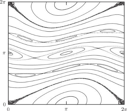
(define window (frame 0.0 :2pi 0.0 :2pi))
(explore-map window (standard-map 0.6) 2000)
The resulting surface of section, for a variety of orbits chosen with the pointer, is shown in figure 3.27. The surface of section does indeed look qualitatively similar to the surfaces of section generated by dynamical systems.
The surface of section for K = 1.4 (as shown in figure 3.28) is dominated by a large chaotic zone. The standard map exhibits a transition to large-scale chaos near K = 1. So this abstract area-preserving map of the phase plane onto itself shows behavior that is similar to behavior in the sections generated by a Hamiltonian dynamical system. Evidently, the area-preservation property of the dynamics in the phase space plays a determining role for many interesting properties of trajectories of mechanical systems.
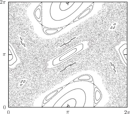
Exercise 3.13: Fun with Hénon's quadratic map
Consider the map of the plane defined by the equations:
x′ = x cos α − (y − x2) sin α
y′ = x sin α + (y − x2) cos α
a. Show that the map preserves area.
b. Implement the map as a procedure. The interesting range of x and y is (−1, 1). There will be orbits that escape. You should check for values of x and y that escape from this range and call the failure continuation when this occurs.
c. Explore the phase portrait of this map for a few values of the parameter α. The map is particularly interesting for α = 1.32 and α = 1.2. What happens in between?
3.10 Summary
Lagrange's equations are a system of n second-order ordinary differential equations in the time, the generalized coordinates, the generalized velocities, and the generalized accelerations. Trajectories are determined by the coordinates and the velocities at a moment.
Hamilton's equations specify the dynamics as a system of first-order ordinary differential equations in the time, the generalized coordinates, and the conjugate momenta. Phase-space trajectories are determined by an initial point in phase space at a moment.
The Hamiltonian formulation and the Lagrangian formulation are equivalent in that equivalent initial conditions produce the same configuration path.
If there is a symmetry of the problem that is naturally expressed as a cyclic coordinate, then the conjugate momentum is conserved. In the Hamiltonian formulation, such a symmetry naturally results in the reduction of the dimension of the phase space of the difficult part of the problem. If there are enough symmetries, then the problem of determining the time evolution may be reduced to evaluation of definite integrals (reduced to quadratures).
Systems without enough symmetries to be reducible to quadratures may be effectively studied with the surface of section technique. This is particularly advantageous in systems for which the reduced problem has two degrees of freedom or has one degree of freedom with explicit periodic time dependence.
Surfaces of section reveal tremendous structure in the phase space. There are chaotic zones and islands of regular behavior. There are interesting transitions as parameters are varied between mostly regular motion and mostly chaotic motion.
Chaotic trajectories exhibit sensitive dependence on initial conditions, separating exponentially from nearby trajectories. Regular trajectories do not show such sensitivity. Curiously, chaotic trajectories are distinguished both by the dimension of the space they explore and by their exponential divergence.
The time evolution of a 2n-dimensional region in phase space preserves the volume. Hamiltonian flow is “incompressible” flow of the “phase fluid.”
Surfaces of section for two-degree-of-freedom systems and for periodically driven one-degree-of-freedom systems are area preserving. Abstract area-preserving maps of a phase plane onto itself show the same division of the phase space into chaotic and regular regions as surfaces of section generated by dynamical systems. They also show transitions to large-scale chaos.
3.11 Projects
Exercise 3.14: Periodically driven pendulum
Explore the dynamics of the driven pendulum, using the surface of section method. We are interested in exploring the regions of parameter space over which various phenomena occur. Consider a pendulum of length 9.8 m, mass 1 kg, and acceleration of gravity g = 9.8 m s−2, giving ω0 = 1 rad s−1. Explore the parameter plane of the amplitude A and frequency ω of the periodic drive.
Examples of the phenomena to be investigated:
a. Inverted equilibrium. Show the region of parameter space (A, ω) in which the inverted equilibrium is stable. If the inverted equilibrium is stable there is some range of stability, i.e., there is a maximum angle of displacement from the equilibrium that stable oscillations reach. If you have enough time, plot contours in the parameter space for different amplitudes of the stable region.
b. Period doubling of the normal equilibrium. For this case, plot the angular momenta of the stable and unstable equilibria as functions of the frequency for some given amplitude.
c. Transition to large-scale chaos. Show the region of parameter space (A, ω) for which the chaotic zones around the three principal resonance islands are linked.
Exercise 3.15: Spin-orbit surfaces of section
Write a program to compute surfaces of section for the spin-orbit problem, with the section points being recorded at pericenter. Investigate the following:
a. Give a Hamiltonian formulation of the spin-orbit problem introduced in section 2.11.2.
b. For out-of-roundness parameter ϵ = 0.1 and eccentricity e = 0.1, measure the widths, in momentum, of the regular islands associated with the 1:1, 3:2, and 1:2 resonances.
c. Explore the surfaces of section for a range of ϵ for fixed e = 0.1. Estimate the critical value of ϵ above which the main chaotic zones around the 3:2 and the 1:1 resonance islands are merged.
d. For a fixed eccentricity e = 0.1 trace the location on the surface of section of the stable and unstable fixed points associated with the 1:1 resonance as a function of the out-of-roundness ϵ.
Exercise 3.16: Restricted three-body problem
Investigate the dynamics of the restricted three-body problem for the equal mass case where M0 = M1.
a. Derive the Hamiltonian for the restricted three-body problem, starting with Lagrangian (1.150).
b. The Jacobi constant, equation (1.151), is the sum of a positive definite quadratic term in the velocities and a potential energy term, equation (1.152), so the boundaries of the allowed motion are contours of the potential energy function. Write a program to display these boundaries for a given value of the Jacobi constant. Where is motion allowed relative to these contours? (Note that for some values of the Jacobi constant there is more than one allowed region of motion.)
c. Evolve some trajectories for a Jacobi constant of ℰ = −1.75 (CJ = 3.5). Display the trajectories on the same plot as the boundaries of allowed motion.
d. Write a program to compute surfaces of section for the restricted three-body problem. This program is similar to the Hénon-Heiles program starting on page 261. Plot section points when the trajectory crosses the yr = 0 axis with ẏr positive; plot ẋr versus xr. Note that px = mẋr − mΩyr, but on this section yr = 0, so the velocity is proportional to the momentum, and thus the section is area preserving. Plot the boundaries of the allowed motion on the surface of section for the Jacobi constant suggested above. Explore the section and plot typical orbits for each major region in the section.
1Here we restrict our attention to Lagrangians that depend only on the time, the coordinates, and the velocities.
2Here we are using mnemonic names t, q, p for formal parameters of the function being defined. We could have used names like a, b, c as above, but this would have made the argument harder to read.
3P = I2. See equations (9.7) in the appendix on notation.
4The overall minus sign in the definition of the Hamiltonian is traditional.
5In traditional notation, Hamilton's equations are written as a separate equation for each component:
6Traditionally, the Hamiltonian is written
This way of writing the Hamiltonian confuses the values of functions with the functions that generate them: both
7In the construction of the Lagrangian state derivative from the Lagrange equations we must solve for the highest-order derivative. The solution process requires the inversion of ∂2∂2L. In the construction of Hamilton's equations, the construction of
8The term phase space was introduced by Josiah Willard Gibbs in his formulation of statistical mechanics. The Hamiltonian plays a fundamental role in the Boltzmann–Gibbs formulation of statistical mechanics and in both the Heisenberg and Schrödinger approaches to quantum mechanics.
9The Legendre transformation is more general than its use in mechanics in that it captures the relationship between conjugate variables in systems as diverse as thermodynamics, circuits, and field theory.
10This can be done so long as the derivative is not zero.
11Equation (3.28) looks like an application of the product rule for derivatives,
12If M is the matrix representation of M, then M = MT.
13The procedure solve-linear-left was introduced in footnote 75 on page 71.
14The function Π[q] is the same as ΠL[q] introduced on page 203. Indeed, the Lagrangian is needed to define momentum in every case, but we are suppressing the dependency here because it does not matter in this argument.
15The variation of the momentum
16It is sometimes asserted that the momenta have a different status in the Lagrangian and Hamiltonian formulations: that in the Hamiltonian framework the momenta are “independent” of the coordinates. From this it is argued that the variations δq and δp are arbitrary and independent, therefore implying that the factor multiplying each of them in the action integral (3.75) must independently be zero, apparently deriving both of Hamilton's equations. The argument is fallacious: we can write δp in terms of δq (see footnote 15).
17In traditional notation the Poisson bracket is written
18For systems with kinetic energy that is quadratic in velocity, this equation does not satisfy the Lipschitz condition at isolated points where the velocity is zero. However the solution for q can be extracted using a definite integral.
19The pendulum has only one unstable equilibrium. Remember that the coordinate is an angle.
20If a Lagrangian does not depend on a particular coordinate then neither does the corresponding Hamiltonian, because the coordinate is a passive variable in the Legendre transform. Such a Hamiltonian is said to be cyclic in that coordinate.
21Traditionally, when a problem has been reduced to the evaluation of a definite integral it is said to be reduced to a “quadrature.” Thus, the determination of the evolution of a cyclic coordinate qi is reduced to a problem of quadrature.
22It is not always possible to choose a set of generalized coordinates in which all symmetries are simultaneously manifest. For these systems, the reduction of the phase space is more complicated. We have already encountered such a problem: the motion of a free rigid body. The system is invariant under rotation about any axis, yet no single coordinate system can reflect this symmetry. Nevertheless, we have already found that the dynamics is described by a system of lower dimension than the full phase space: the Euler equations.
23The surface of section technique was introduced by Poincaré in his Méthodes Nouvelles de la Mécanique Céleste [35]. Poincaré proved remarkable results about dynamical systems using the surface of section technique, and we shall return to some of these later. The surface of section technique is a key tool in the modern study of dynamical systems, for both analytical and numerical investigations.
24That solutions of ordinary differential equations can show exponential sensitivity to initial conditions was independently discovered by Edward Lorenz [31] in the context of a simplified model of convection in the Earth's atmosphere. Lorenz coined the picturesque term “butterfly effect” to describe this sensitivity: his weather system model is so sensitive to initial conditions that “the flapping of a butterfly's wings in Brazil can change the course of a typhoon in Japan.”
25We saw an example of this extreme sensitivity to initial conditions in figure 1.7 (section 1.7) and also in the double-pendulum project (exercise 1.44).
26One-dimensional invariant sets with an infinite number of holes were discovered by John Mather. They are sometimes called cantori (singular cantorus), by analogy to the Cantor sets, but it really doesn't Mather.
27In the particular case of the driven pendulum there is no reason to call fail. This contingency is reserved for systems where orbits escape or cease to satisfy some constraint.
28We will see that it is convenient to look at distribution functions in the phase-space coordinates because the consequences of conserved momenta are more apparent, and also because volume in phase space is conserved by evolution (see section 3.8).
29A system is ergodic if time averages along trajectories are the same as phase-space averages over the region explored by the trajectories.
30As before, upon close examination we may find that trajectories that appear to be confined to a curve on the section are chaotic trajectories that explore a highly confined region. It is known, however, that some trajectories really are confined to curves on the section. Trajectories that start on these curves remain on these curves forever, and they fill these curves densely. These invariant curves are preserved by the dynamical evolution. There are also invariant subsets of curves with an infinite number of holes.
31In strongly chaotic systems ζ(t) may become so large that the computer can no longer represent it. To prevent this we can replace ζ by ζ/c whenever ζ(t) becomes uncomfortably large. The equation governing ζ is linear, so except for the scale change, the evolution is unchanged. Of course we have to keep track of these scale changes when computing the average growth rate. This process is called “renormalization” to make it sound impressive.
32The separatrix is the curve that separates the oscillating motion from the circulating motion. It is made up of several trajectories that are asymptotic to the unstable equilibrium.
33It is reported that when Boltzmann was confronted with this problem he responded, “You should wait that long!”
34This is just the product of the Lagrangian for the undamped harmonic oscillator with an increasing exponential of time.
35This question was also addressed in the remarkable paper by Hénon and Heiles, but with a different map from what we use here.
36The standard map has been extensively studied. Early investigations were by Chirikov [12] and by Taylor [44], so the map is sometimes called the Chirikov–Taylor map. Chirikov coined the term “standard map,” which we adopt.