5Canonical Transformations
We have done considerable mountain climbing. Now we are in the rarefied atmosphere of theories of excessive beauty and we are nearing a high plateau on which geometry, optics, mechanics, and wave mechanics meet on common ground. Only concentrated thinking, and a considerable amount of re–creation, will reveal the beauty of our subject in which the last word has not been spoken.
Cornelius Lanczos, The Variational Principles of Mechanics [29], p. 229
One way to simplify the analysis of a problem is to express it in a form in which the solution has a simple representation. However, it may not be easy to formulate the problem in such a way initially. It is often useful to start by formulating the problem in one way, and then transform it. For example, the formulation of the problem of the motion of a number of gravitating bodies is simple in rectangular coordinates, but it is easier to understand aspects of the motion in terms of orbital elements, such as the semimajor axes, eccentricities, and inclinations of the orbits. The semimajor axis and eccentricity of an orbit depend on both the configuration and the velocity of the body. Such transformations are more general than those that express changes in configuration coordinates. Here we investigate transformations of phase-space coordinates that involve both the generalized coordinates and the generalized momenta.
Suppose we have two different Hamiltonian systems, and suppose the trajectories of the two systems are in one-to-one correspondence. In this case both Hamiltonian systems can be mathematical models of the same physical system. Some questions about the physical system may be easier to answer by reference to one model and others may be easier to answer in the other model. For example, it may be easier to formulate the physical system in one model and to discover a conserved quantity in the other. Canonical transformations are maps between Hamiltonian systems that preserve the dynamics.
A canonical transformation is a phase-space coordinate transformation and an associated transformation of the Hamiltonian such that the dynamics given by Hamilton's equations in the two representations describe the same evolution of the system.
5.1 Point Transformations
A point transformation is a canonical transformation that extends a possibly time-dependent transformation of the configuration coordinates to a phase-space transformation. For example, one might want to reexpress motion in terms of polar coordinates, given a description in terms of rectangular coordinates. In order to extend a transformation of the configuration coordinates to a phase-space transformation we must specify how the momenta and Hamiltonian are transformed.
We have already seen how coordinate transformations can be carried out in the Lagrangian formulation (see section 1.6.1). In that case, we found that if the Lagrangian transforms by composition with the coordinate transformation, then the Lagrange equations are equivalent.
Lagrangians that differ by the addition of a total time derivative have the same Lagrange equations, but may have different momenta conjugate to the generalized coordinates. So there is more than one way to make a canonical extension of a coordinate transformation.
Here, we find the particular canonical extension of a coordinate transformation for which the Lagrangians transform by composition with the transformation, with no extra total time derivative terms added to the Lagrangian.
Let L be a Lagrangian for a system. Consider the coordinate transformation q = F (t, q′). The velocities transform by
We obtain a Lagrangian L′ in the transformed coordinates by composition of L with the coordinate transformation. We require that L′(t, q′, v′) = L(t, q, v), so:
The momentum conjugate to q′ is
where we have used
We can collect these results to define a canonical phase-space transformation CH:2
The Hamiltonian is obtained by the Legendre transform
using relations (5.1) and (5.3) in the second step. Fully expressed in terms of the transformed coordinates and momenta, the transformed Hamiltonian is
The Hamiltonians H′ and H are equivalent because L and L′ have the same value for a given dynamical state and so have the same paths of stationary action. In general H and H′ do not have the same values for a given dynamical state, but differ by a term that depends on the coordinate transformation.
For time-independent transformations, ∂0F = 0, there are a number of simplifications. The relationship of the velocities (5.1) becomes
Comparing this to the relation (5.5) between the momenta, we see that in this case the momenta transform “oppositely” to the velocities3
so the product of the momenta and the velocities is not changed by the transformation. This, combined with the fact that by construction L(t, q, v) = L′(t, q′, v′), shows that
For time-independent coordinate transformations the Hamiltonian transforms by composition with the associated phase-space transformation. We can also see this from the general relationship (5.7) between the Hamiltonians.
Implementing point transformations
The procedure F->CH takes a procedure F implementing a transformation of configuration coordinates and returns a procedure implementing a transformation of phase-space coordinates:4
(define ((F->CH F) state)
  (up (time state)
      (F state)
      (solve-linear-right
        (momentum state)
        (((partial 1) F) state))))
Consider a particle moving in a central field. In rectangular coordinates a Hamiltonian is
(define ((H-central m V) state)
  (let ((x (coordinate state))
        (p (momentum state)))
    (+ (/ (square p) (* 2 m))
       (V (sqrt (square x))))))
Let's look at this Hamiltonian in polar coordinates. The phase-space transformation is obtained by applying F->CH to the procedure p->r that takes a time and a polar tuple and returns a tuple of rectangular coordinates (see section 1.6.1). The transformation is time independent so the Hamiltonian transforms by composition. In polar coordinates the Hamiltonian is
(show-expression
  ((compose
     (H-central 'm (literal-function 'V))
     (F->CH p->r))
(up 't (up 'r 'phi) (down 'p_r 'p_phi))))There are three terms. There is the potential energy, which depends on the radius, there is the kinetic energy due to radial motion, and there is the kinetic energy due to tangential motion. As expected, the angle φ does not appear and thus the angular momentum is a conserved quantity. By going to polar coordinates we have decoupled one of the two degrees of freedom in the problem.
If the transformation is time varying the Hamiltonian must be adjusted by adding a correction to the composition of the Hamiltonian and the transformation (see equation 5.8):
The correction is computed by
(define ((F->K F) state)
  (- (* (solve-linear-right
          (momentum state)
          (((partial 1) F) state))
        (((partial 0) F) state))))
For example, consider a transformation to coordinates translating with velocity v:
(define ((translating v) state)
  (+ (coordinates state) (* v (time state))))
We compute the additive adjustment required for the Hamiltonian:
((F->K (translating (up 'v^x 'v^y 'v^z)))
(up 't (up 'x 'y 'z) (down 'p_x 'p_y 'p_z)))(+ (* -1 p_x v^x) (* -1 p_y v^y) (* -1 p_z v^z))Notice that this is the negation of the inner product of the momentum and the velocity of the coordinate system.
Let's see how a simple free-particle Hamiltonian is transformed:
(define ((H-free m) s)
(/ (square (momentum s)) (* 2 m)))
The transformed Hamiltonian is:
(define H-prime
  (+ (compose (H-free 'm)
              (F->CH (translating (up 'v^x 'v^y 'v^z))))
(F->K (translating (up 'v^x 'v^y 'v^z)))))(H-prime
(up 't
(up 'xprime 'yprime 'zprime)
(down 'pprime_x 'pprime_y 'pprime_z)))
(+ (* -1 pprime_x v^x)
(* -1 pprime_y v^y)
(* -1 pprime_z v^z)
(/ (* 1/2 (expt pprime_x 2)) m)
(/ (* 1/2 (expt pprime_y 2)) m)
(/ (* 1/2 (expt pprime_z 2)) m))Exercise 5.1: Galilean invariance
Is this result what you expected? Let's investigate.
Recall that in exercise 1.29 we showed that if the kinetic energy is
Let CH be the phase space extension of the translation transformation, and C be the local tuple extension. The transformed Hamiltonian is H′ = H ∘ CH + K; the transformed Lagrangian is L′ = L ∘ C.
a. Derive the relationship between p and p′ both from CH and from the Lagrangians. Are they the same? Derive the relationship between v and v′ by taking the derivative of the Hamiltonians with respect to the momenta (Hamilton's equation). Show that the Legendre transform of L′ gives the same H′.
b. We have shown that L and L′ differ by a total time derivative. So for any uniformly moving coordinate system we can write the Lagrangian as
Exercise 5.2: Rotations
Let q and q′ be rectangular coordinates that are related by a rotation R: q = Rq′. The Lagrangian for the system is
5.2 General Canonical Transformations
Although we have shown how to extend any coordinate transformation of the configuration space to a canonical transformation, there are other ways to construct canonical transformations. How do we know if we have a canonical transformation? To test if a transformation is canonical we may use the fact that if the transformation is canonical, then Hamilton's equations of motion for the transformed system and the original system will be equivalent.
Consider a Hamiltonian H and a phase-space transformation CH. Let Ds be the function that takes a Hamiltonian and gives the Hamiltonian state-space derivative:5
Hamilton's equations are
for any realizable phase-space path σ.
The transformation CH transforms the phase-space path σ′ (t) = (t, q′ (t), p′ (t)) into σ(t) = (t, q(t), p(t)):
The rates of change of the phase-space coordinates are transformed by the derivative of the transformation
The transformation is canonical if the equations of motion obtained from the new Hamiltonian are the same as those that could be obtained by transforming the equations of motion derived from the original Hamiltonian to the new coordinates:
Using equation (5.14), we see that
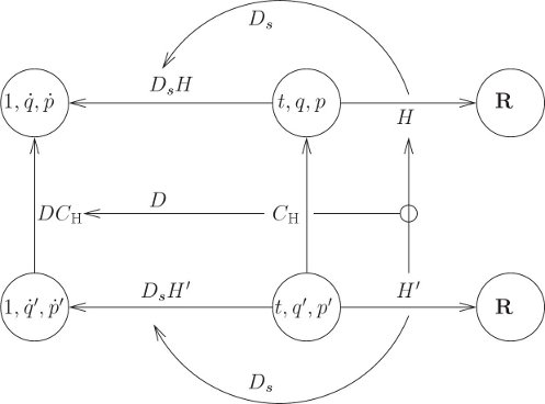
With σ = CH ∘ σ′, we find
This condition must hold for any realizable phase-space path σ′. Certainly this is true if the following condition holds for every phase-space point:6
Any transformation that satisfies equation (5.20) is a canonical transformation among phase-space representations of a dynamical system. In one phase-space representation the system's dynamics is characterized by the Hamiltonian H′ and in the other by H. The idea behind this equation is illustrated in figure 5.1.
We can formalize this test as a program:
(define (canonical? C H Hprime)
  (- (compose (Hamiltonian->state-derivative H) C)
     (* (D C) (Hamiltonian->state-derivative Hprime))))
where Hamiltonian->state-derivative, which was introduced in chapter 3, implements Ds. The transformation is canonical if these residuals are zero.
For time-independent point transformations an appropriate Hamiltonian can be formed by composition with the corresponding phase-space transformation. For more general canonical transformations, we will see that if a transformation is independent of time, a suitable Hamiltonian for the transformed system can be obtained by composing the Hamiltonian with the phase-space transformation. In this case we obtain a more specific formula:
Polar-canonical transformation
The analysis of the harmonic oscillator illustrates the use of a general canonical transformation in the solution of a problem. The harmonic oscillator is a mathematical model of a simple spring-mass system. A Hamiltonian for a spring-mass system with mass m and spring constant k is
Hamilton's equations of motion are
giving the second-order system
The solution is
where
and where A and φ are determined by initial conditions.
We use the polar-canonical transformation:
where
Here α is an arbitrary parameter. We define:
(define ((polar-canonical alpha) state)
  (let ((t (time state))
        (theta (coordinate state))
        (I (momentum state)))
    (let ((x (* (sqrt (/ (* 2 I) alpha)) (sin theta)))
          (p_x (* (sqrt (* 2 alpha I)) (cos theta))))
      (up t x p_x))))
And now we just run our test:
(define ((H-harmonic m k) s)
  (+ (/ (square (momentum s)) (* 2 m))
     (* 1/2 k (square (coordinate s)))))

((canonical?
   (polar-canonical 'alpha)
   (H-harmonic 'm 'k)
   (compose (H-harmonic 'm 'k)
            (polar-canonical 'alpha)))
(up 't 'theta 'I))(up 0 0 0)So the transformation is canonical for the harmonic oscillator.7
Let's use our polar-canonical transformation Cα to help us solve the harmonic oscillator. We substitute expressions (5.28) and (5.29) for x and px in the Hamiltonian, getting our new Hamiltonian:
If we choose
and the new Hamiltonian no longer depends on the coordinate. Hamilton's equation for I is
so I is constant. The equation for θ is
so
In the original variables,
with the constant
Exercise 5.3: Trouble in Lagrangian world
Is there a Lagrangian L′ that corresponds to the harmonic oscillator Hamiltonian H′(t, θ, I) = ωI? What could this possibly mean?
Exercise 5.4: Group properties
If we say that CH is canonical with respect to Hamiltonians H and H′ if and only if DsH ∘ CH = DCH · DsH′, then:
a. Show that the composition of canonical transformations is canonical.
b. Show that composition of canonical transformations is associative.
c. Show that the identity transformation is canonical.
d. Show that there is an inverse for a canonical transformation and the inverse is canonical.
5.2.1 Time-Dependent Transformations
We have seen that for time-dependent point transformations the Hamiltonian appropriate for the transformed system is the original Hamiltonian composed with the transformation and augmented with an additive correction. Here we find a similar decomposition for general time-dependent canonical transformations.
The key to this decomposition is to separate the time part and the phase-space part of the Hamiltonian state derivative:8
where
as code:9
(define (T-func s)
  (up 1
      (zero-like (coordinates s))
      (zero-like (momenta s))))

(define ((D-phase-space H) s)
  (up 0 (((partial 2) H) s) (- (((partial 1) H) s))))
If we assume that H′ = H ∘ CH + K, then the canonical condition (5.20) becomes
Expanding the state derivative, the canonical condition is
Equation (5.40) is satisfied if the following conditions are met:
The value of T ∘ CH does not depend on CH, so this term is really very simple. Notice that equation (5.41) does not depend upon K and that equation (5.42) does not depend upon H.
These can be implemented as follows:
(define (canonical-H? C H)
  (- (compose (D-phase-space H) C)
     (* (D C)
        (D-phase-space (compose H C)))))

(define (canonical-K? C K)
  (- (compose T-func C)
     (* (D C)
        (+ T-func (D-phase-space K)))))
Rotating coordinates
Consider a time-dependent transformation to uniformly rotating coordinates:10
with components
As a program this is
(define ((rotating Omega) state)
  (let ((t (time state)) (qp (coordinate state)))
    (let ((xp (ref qp 0)) (yp (ref qp 1)) (zp (ref qp 2)))
      (up (- (* (cos (* Omega t)) xp)
             (* (sin (* Omega t)) yp))
          (+ (* (sin (* Omega t)) xp)
             (* (cos (* Omega t)) yp))
          zp))))
The extension of this transformation to a phase-space transformation is
(define (C-rotating Omega) (F->CH (rotating Omega)))We first verify that this time-dependent transformation satisfies equation (5.41). We will try it for an arbitrary Hamiltonian with three degrees of freedom:
(define H-arbitrary
  (literal-function 'H
                    (-> (UP Real (UP Real Real Real) (DOWN Real Real Real))
                        Real)))

((canonical-H? (C-rotating 'Omega) H-arbitrary)
 (up 't (up 'xp 'yp 'zp) (down 'pp_x 'pp_y 'pp_z)))
(up 0 (up 0 0 0) (down 0 0 0))
And it works. Note that this result did not depend on any details of the Hamiltonian, suggesting that we might be able to make a test that does not require a Hamiltonian. We will see that shortly.
Since we have a point transformation, we can compute the required adjustment to the Hamiltonian:
((F->K (rotating 'Omega))
 (up 't (up 'xp 'yp 'zp) (down 'pp_x 'pp_y 'pp_z)))
(+ (* Omega pp_x yp) (* -1 Omega pp_y xp))
So, for this transformation an appropriate correction to the Hamiltonian is
which is minus the rate of rotation of the coordinate system multiplied by the angular momentum. We implement K as a procedure
(define ((K Omega) s)
  (let ((qp (coordinate s)) (pp (momentum s)))
    (let ((xp (ref qp 0)) (yp (ref qp 1))
                          (ppx (ref pp 0)) (ppy (ref pp 1)))
      (* -1 Omega (- (* xp ppy) (* yp ppx))))))
and apply the test. We find:
((canonical-K? (C-rotating 'Omega) (K 'Omega))
 (up 't (up 'xp 'yp 'zp) (down 'pp_x 'pp_y 'pp_z)))
(up 0 (up 0 0 0) (down 0 0 0))
The residuals are zero so this K correctly completes the canonical transformation.
5.2.2 Abstracting the Canonical Condition
We just saw that for the case of rotating coordinates the truth of equation (5.41) did not depend on the details of the Hamiltonian. If CH satisfies equation (5.41) for any H then we can derive a condition on CH that is independent of H.
Let's start with an expanded version of equation (5.41):
using the chain rule.
We introduce a shuffle function:
The argument to
Let J be the multiplier corresponding to the constant linear function
where s⋆ is an arbitrary argument, shaped like DH(s), that is compatible for multiplication with s. The value of s⋆ is irrelevant because D
We can move the DCH(s′) to the left of DH(CH(s′)) by taking its transpose:11
Since
This is true for any H if
(define (J-func DHs)
  (up 0 (ref DHs 2) (- (ref DHs 1))))

(define ((canonical-transform? C) s)
  (let ((J ((D J-func) (compatible-shape s)))
        (DCs ((D C) s)))
    (- J (* DCs J (transpose DCs s)))))
This condition, equation (5.52), on CH, called the canonical condition, does not depend on the details of H. This is a remarkable result: we can decide whether a phase-space transformation preserves the dynamics of Hamilton's equations without further reference to the details of the dynamical system. If the transformation is time dependent we can add a correction to the Hamiltonian to make it canonical.
Examples
The polar-canonical transformation satisfies the canonical condition:
((canonical-transform? (polar-canonical 'alpha))
 (up 't 'theta 'I))
(up (up 0 0 0) (up 0 0 0) (up 0 0 0))
But not every transformation we might try satisfies the canonical condition. For example, we might try x = p sin θ and px = p cos θ. The implementation is
(define (a-non-canonical-transform state)
  (let ((t (time state))
        (theta (coordinate state))
        (p (momentum state)))
    (let ((x (* p (sin theta)))
          (p_x (* p (cos theta))))
      (up t x p_x))))

((canonical-transform? a-non-canonical-transform)
 (up 't 'theta 'p))
(up (up 0 0 0) (up 0 0 (+ -1 p)) (up 0 (+ 1 (* -1 p)) 0))
So this transformation does not satisfy the canonical condition.
Canonical condition and Poisson brackets
The canonical condition can be written simply in terms of Poisson brackets.
The Poisson bracket can be written in terms of
as can be seen by writing out the components.
We break the transformation CH into position and momentum parts:
In terms of the individual component functions, the canonical condition (5.52) is
where
We have found that a transformation is canonical if its position-momentum part satisfies the canonical condition, but for a time-dependent transformation we may have to modify the Hamiltonian by the addition of a suitable K. We can rewrite these conditions in terms of Poisson brackets. If the Hamiltonian is
the transformation will be canonical if the coordinate-momentum transformation satisfies the fundamental Poisson brackets, and K satisfies:
Exercise 5.5: Poisson bracket conditions
Fill in the details to show that the canonical condition (5.52) is equivalent to the fundamental Poisson brackets (5.56) and that the condition on K (5.42) is equivalent to the Poisson bracket condition on K (5.58).
Symplectic matrices
It is convenient to reformulate the canonical condition in terms of matrices. We can obtain a matrix representation of a structure with the utility s->m that takes a structure that represents a multiplier of a linear transformation and returns a matrix representation of the multiplier. The procedure s->m takes three arguments: (s->m ls A rs). The ls and rs specify the shapes of objects that multiply A on the left and right to give a numerical value. These specify the basis. So, the matrix representation of the multiplier corresponding to
(let* ((s (up 't (up 'x 'y) (down 'px 'py)))
       (s* (compatible-shape s))
       (J ((D J-func) s*)))
(s->m s* J s*))(matrix-by-rows
(list 0 0 0 0 0)
(list 0 0 0 1 0)
(list 0 0 0 0 1)
(list 0 -1 0 0 0)
(list 0 0 -1 0 0))This matrix, J, is useful, so we supply a procedure J-matrix so that (J-matrix n) gives this matrix for an n degree-of-freedom system.
We can now reexpress the canonical condition (5.52) as a matrix equation:
There is a further simplification available. The elements of the first row and the first column of the matrix representation of
(define C-general
  (literal-function 'C
                    (-> (UP Real (UP Real Real) (DOWN Real Real))
                        (UP Real (UP Real Real) (DOWN Real Real)))))
Consider transformations for which the time does not depend on the coordinates or momenta14
(define (C-simple-time s)
  (let ((cs (C-general s)))
    (up ((literal-function 'tau) (time s))
        (coordinates cs)
        (momenta cs))))
For this kind of transformation the first row and the first column of the residuals of the canonical-transform? test are identically zero:
(let* ((s (up 't (up 'x 'y) (down 'p_x 'p_y)))
       (s* (compatible-shape s)))
  (m:nth-row
    (s->m s* ((canonical-transform? C-simple-time) s) s*)
0))(up 0 0 0 0 0)(let ((s (up 't (up 'x 'y) (down 'p_x 'p_y)))
(s* (compatible-shape s)))
(m:nth-col
(s->m s* ((canonical-transform? C-simple-time) s) s*)
0))(up 0 0 0 0 0)But for C-general these are not zero. Since the transformations we are considering at most shift time, we need to consider only the submatrix associated with the coordinates and the momenta.
The qp submatrix15 of dimension 2n × 2n of the matrix J is called the symplectic unit for n degrees of freedom:
The matrix Jn satisfies the following identities:
A 2n × 2n matrix A that satisfies the relation
is called a symplectic matrix. We can determine whether a matrix is symplectic:
(define (symplectic-matrix? M)
  (let ((2n (m:dimension M)))
    (let ((J (symplectic-unit (quotient 2n 2))))
      (- J (* M J (transpose M))))))
An appropriate symplectic unit matrix of a given size is produced by the procedure symplectic-unit.
If the matrix representation of the derivative of a transformation is a symplectic matrix the transformation is a symplectic transformation. Here is a test for whether a transformation is symplectic:16
(define ((symplectic-transform? C) s)
  (symplectic-matrix? (qp-submatrix ((D-as-matrix C) s))))
The procedure symplectic-transform? returns a zero matrix if and only if the transformation being tested passes the symplectic matrix test.
For example, the point transformations are symplectic. We can show this for a general possibly time-dependent two-degree-of-freedom point transformation:
(define (F s)
  ((literal-function 'F
                     (-> (X Real (UP Real Real)) (UP Real Real)))
   (time s) (coordinates s)))

((symplectic-transform? (F->CH F))
(up 't (up 'x 'y) (down 'px 'py)))(matrix-by-rows
(list 0 0 0 0)
(list 0 0 0 0)
(list 0 0 0 0)
(list 0 0 0 0))More generally, the phase-space part of the canonical condition is equivalent to the symplectic condition (for two degrees of freedom) even in the case of an unrestricted phase-space transformation.
(let* ((s (up 't (up 'x 'y) (down 'p_x 'p_y)))
       (s* (compatible-shape s)))
  (- (qp-submatrix
       (s->m s* ((canonical-transform? C-general) s) s*))
((symplectic-transform? C-general) s)))(matrix-by-rows
(list 0 0 0 0)
(list 0 0 0 0)
(list 0 0 0 0)
(list 0 0 0 0))Exercise 5.6: Symplectic matrices
Let A be a symplectic matrix:
Exercise 5.7: Polar-canonical transformations
Let x, p and θ, I be two sets of canonically conjugate variables. Consider transformations of the form x = βIα sin θ and p = βIα cos θ. Determine all α and β for which this transformation is symplectic.
Exercise 5.8: Standard map
Is the standard map a symplectic transformation? Recall that the standard map is: I′ = I + K sin θ, with θ′ = θ + I′, both modulo 2π.
Exercise 5.9: Whittaker transform
Shew that the transformation q = log ((sin p′)/q′) with p = q′ cot p′ is symplectic.
5.3 Invariants of Canonical Transformations
Canonical transformations allow us to change the phase-space coordinate system that we use to express a problem, preserving the form of Hamilton's equations. If we solve Hamilton's equations in one phase-space coordinate system we can use the transformation to carry the solution to the other coordinate system. What other properties are preserved by a canonical transformation?
Noninvariance of pv
We noted in equation (5.10) that point transformations that are canonical extensions of time-independent coordinate transformations preserve the value of pv. This does not hold for more general canonical transformations. We can illustrate this with the polar-canonical transformation. Along corresponding paths x, px and θ, I
and so Dx is
The difference of pv and the transformed p′v′ is
In general this is not zero. So the product pv is not necessarily invariant under general canonical transformations.
Invariance of Poisson brackets
Here is a remarkable fact: the composition of the Poisson bracket of two phase-space state functions with a canonical transformation is the same as the Poisson bracket of each of the two functions composed with the transformation separately. Loosely speaking, the Poisson bracket is invariant under canonical phase-space transformations.
Let f and g be two phase-space state functions. Using the
where the fact that CH satisfies equation (5.41) was used in the middle. This is
Volume preservation
Consider a canonical transformation CH. Let Ĉt be a function with parameter t such that (q, p) = Ĉt(q′, p′) if (t, q, p) = CH(t, q′, p′). The function Ĉt maps phase-space coordinates to alternate phase-space coordinates at a given time. Consider regions R in (q, p) and R in (q′, p′) such that R = Ĉt(R′). The volume of region R′ is
where
Thus, phase-space volume is preserved by symplectic transformations.
Liouville's theorem shows that time evolution preserves phase-space volume. Here we see that canonical transformations also preserve phase volumes. Later, we will find that time evolution actually generates a canonical transformation.
The symplectic 2-form
Define
where Q = I1 and P = I2 are the coordinate and momentum selectors, respectively. The arguments ζ1 and ζ2 are incremental phase-space states with zero time components.
The ω form can also be written as a sum over degrees of freedom:
Notice that the contributions for each i do not mix components from different degrees of freedom.
This bilinear form is closely related to the symplectic 2-form of differential geometry. It differs in that the symplectic 2-form is formally a function of the phase-space point as well as the incremental vectors.
Under a canonical transformation s = CH(s′), incremental states transform with the derivative
We will show that the 2-form is invariant under this transformation
if the time components of the
We have shown that condition (5.41) does not depend on the details of the Hamiltonian H. So if a transformation satisfies the canonical condition we can use condition (5.41) with H replaced by an arbitrary function f of phase-space states:
In terms of ω, the Poisson bracket is
as can be seen by writing out the components. We use the fact that Poisson brackets are invariant under canonical transformations:
Using the relation (5.74) to expand the left-hand side of equation (5.76) we obtain:
The right-hand side of equation (5.76) is
Now the left-hand side must equal the right-hand side for any f and g, so the equation must also be true for arbitrary
So the
We have proven that
for canonical CH and incremental states
Thus the bilinear antisymmetric function ω is invariant under even time-varying canonical transformations if the increments are restricted to have zero time component.
As a program, ω is
(define (omega zeta1 zeta2)
  (- (* (momentum zeta2) (coordinate zeta1))
     (* (momentum zeta1) (coordinate zeta2))))
On page 356 we showed that point transformations are sym-plectic. Here we can see that the 2-form is preserved under these transformations for two degrees of freedom:
(define (F s)
  ((literal-function 'F
                     (-> (X Real (UP Real Real)) (UP Real Real)))
   (time s)
   (coordinates s)))

(let ((s (up 't (up 'x 'y) (down 'p_x 'p_y)))
      (zeta1 (up 0 (up 'dx1 'dy1) (down 'dp1_x 'dp1_y)))
      (zeta2 (up 0 (up 'dx2 'dy2) (down 'dp2_x 'dp2_y))))
  (let ((DCs ((D (F->CH F)) s)))
    (- (omega zeta1 zeta2)
       (omega (* DCs zeta1) (* DCs zeta2)))))
0
Alternatively, let z1 and z2 be the matrix representations of the qp parts of ζ1 and ζ2. The matrix representation of ω is
Let A be the matrix representation of the qp part of DCH(s′) Then the invariance of ω is equivalent to
But this is true if
which is equivalent to the condition that A is symplectic. (If a matrix is symplectic then its transpose is symplectic. See exercise 5.6).
The symplectic condition is symmetrical in that if A is symplec-tic then
is satisfied by time-varying canonical transformations, and time-varying canonical transformations are symplectic. But if the transformation is time varying then
is not satisfied because J is not invertible. Equation (5.86) is satisfied, however, for time-independent transformations.
Poincaré integral invariant
The invariance of the symplectic 2-form under canonical transformations has a simple interpretation. Consider how the area of an incremental parallelogram in phase space transforms under canonical transformation. Let (Δq, Δp) and (δq, δp) be small increments in phase space, originating at (q, p). Consider the incremental parallelogram with vertex at (q, p) with these two phase-space increments as edges. The sum of the areas of the canonical projections of this incremental parallelogram can be written
The right-hand side is the sum of the areas on the canonical planes;17 for each i the area of a parallelogram is computed from the components of the vectors defining its adjacent sides. Let ζ1 = (0, Δq, Δp) and ζ2 = (0, δq, δp); then the sum of the areas of the incremental parallelograms is just
where ω is the bilinear antisymmetric function introduced in equation (5.70). The function ω is invariant under canonical transformations, so the sum of the areas of the incremental parallelograms is invariant under canonical transformations.
There is an integral version of this differential relation. Consider the oriented area of a region R′ in phase space (see figure 5.2). Suppose we make a canonical transformation from coordinates (q′, p′) to (q, p) taking region R′ to region R. The boundary of the region in the transformed coordinates is just the image under the canonical transformation of the original boundary. Let
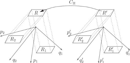
The area of an arbitrary region is just the limit of the sum of the areas of incremental parallelograms that cover the region, so the sum of oriented areas is preserved by canonical transformations:
That is, the sum of the projected areas on the canonical planes is preserved by canonical transformations. Another way to say this is
The equality-of-areas relation (5.90) can also be written as an equality of line integrals using Stokes's theorem, for simply-connected regions
The canonical planes are disjoint except at the origin, so the projected areas intersect in at most one point. Thus we may independently accumulate the line integrals around the boundaries of the individual projections of the region onto the canonical planes into a line integral around the unprojected region:
Exercise 5.10: Watch out
Consider the canonical transformation CH:
a. Show that the transformation is symplectic for any a.
b. Show that equation (5.92) is not generally satisfied for the region enclosed by a curve of constant J.
5.4 Generating Functions
We have considered a number of properties of general canonical transformations without having a method for coming up with them. Here we introduce the method of generating functions. The generating function is a real-valued function that compactly specifies a canonical transformation through its partial derivatives, as follows.
Consider a real-valued function F1(t, q, q′) mapping configurations expressed in two coordinate systems to the reals. We will use F1 to construct a canonical transformation from one coordinate system to the other. We will show that the following relations among the coordinates, the momenta, and the Hamiltonians specify a canonical transformation:
The transformation will then be explicitly given by solving for one set of variables in terms of the others: To obtain the primed variables in terms of the unprimed ones, let A be the inverse of ∂1F1 with respect to the third argument,
then
Let B be the coordinate part of the phase-space transformation q = B(t, q′, p′). This B is an inverse function of ∂2F1, satisfying
Using B, we have
To put the transformation in explicit form requires that the inverse functions A and B exist.
We can use the above relations to verify that some given transformation from one set of phase-space coordinates (q, p) with Hamiltonian function H(t, q, p) to another set (q′, p′) with Hamiltonian function H′(t, q′, p′) is canonical by finding an F1(t, q, q′) such that the above relations are satisfied. We can also use arbitrarily chosen generating functions of type F1 to generate new canonical transformations.
The polar-canonical transformation
The polar-canonical transformation (5.27) from coordinate and momentum (x, px) to new coordinate and new momentum (θ, I),
introduced earlier, is canonical. This can also be demonstrated by finding a suitable F1 generating function. The generating function satisfies a set of partial differential equations, (5.93) and (5.94):
Using relations (5.102) and (5.103), which specify the transformation, equation (5.104) can be rewritten
which is easily integrated to yield
where φ is some integration “constant” with respect to the first integration. Substituting this form for F1 into the second partial differential equation (5.105), we find
but if we set φ = 0 the desired relations are recovered. So the generating function
generates the polar-canonical transformation. This shows that this transformation is canonical.
5.4.1 F1 Generates Canonical Transformations
We can prove directly that the transformation generated by an F1 is canonical by showing that if Hamilton's equations are satisfied in one set of coordinates then they will be satisfied in the other set of coordinates. Let F1 take arguments (t, x, y). The relations among the coordinates are
and the Hamiltonians are related by
Substituting the generating function relations (5.110) into this equation, we have
Take the partial derivatives of this equality of expressions with respect to the variables x and y:18
where the arguments are unambiguous and have been suppressed. On solution paths we can use Hamilton's equations for the (x, px) system to replace the partial derivatives of H with derivatives of x and px, obtaining
Now compute the derivatives of px and py, from equations (5.110), along consistent paths:
Using the fact that elementary partials commute, (∂2(∂1F1)i)j = (∂1(∂2F1)j)i, and substituting this expression for (Dpx)i into the first of equations (5.114) yields
Provided that ∂2∂1F1 is nonsingular,19 we have derived one of Hamilton's equations for the (y, py) system:
Hamilton's other equation,
can be derived in a similar way. So the generating function relations indeed specify a canonical transformation.
5.4.2 Generating Functions and Integral Invariants
Generating functions can be used to specify a canonical transformation by the prescription given above. Here we show how to get a generating function from a canonical transformation, and derive the generating function rules.
The generating function representation of canonical transformations can be derived from the Poincaré integral invariants, as follows. We first show that, given a canonical transformation, the integral invariants imply the existence of a function of phase-space coordinates that can be written as a path-independent line integral. Then we show that partial derivatives of this function, represented in mixed coordinates, give the generating function relations between the old and new coordinates. We need to do this only for time-independent transformations because time-dependent transformations become time independent in the extended phase space (see section 5.5).
Generating functions of type F1
Let C be a time-independent canonical transformation, and let Ct be the qp-part of the transformation. The transformation Ct preserves the integral invariant equation (5.90). One way to express the equality of areas is as a line integral (5.92):
where R′ is a two-dimensional region in (q′, p′) coordinates at time t, R = Ct(R′) is the corresponding region in (q, p) coordinates, and ∂R indicates the boundary of the region R. This holds for any region and its boundary. We will show that this implies there is a function F (t, q′, p′) that can be defined in terms of line integrals
where γ′ is a curve in phase-space coordinates that begins at
Let
and let
So the value of Gt(γ′) depends only on the endpoints of γ′.
Let
where γ′ is any path from
If we define F so that
then
demonstrating equation (5.120).
The phase-space point (q, p) in unprimed variables corresponds to (q′, p′) in primed variables, at an arbitrary time t. Both p and q are determined given q′ and p′. In general, given any two of these four quantities, we can solve for the other two. If we can solve for the momenta in terms of the positions we get a particular class of generating functions.20 We introduce the functions
that solve the transformation equations (t, q, p) = C(t, q′, p′) for the momenta in terms of the coordinates at a specified time. With these we introduce a function F1(t, q, q′) such that
The function F1 has the same value as F but has different arguments. We will show that this F1 is in fact the generating function for canonical transformations introduced in section 5.4. Let's be explicit about the definition of F1 in terms of a line integral:
The two line integrals can be combined into this one because they are both expressed as integrals along a curve in (q, q′).
We can use the path independence of F1 to compute the partial derivatives of F1 with respect to particular components and consequently derive the generating function relations for the momenta.21 So we conclude that
These are just the configuration and momentum parts of the generating function relations for canonical transformation. So starting with a canonical transformation, we can find a generating function that gives the coordinate–momentum part of the transformation through its derivatives.
Starting from a general canonical transformation, we have constructed an F1 generating function from which the canonical transformation may be rederived. So we expect there is a generating function for every canonical transformation.22
Generating functions of type F2
Point transformations were excluded from the previous argument because we could not deduce the momenta from the coordinates. However, a similar derivation allows us to make a generating function for this case. The integral invariants give us an equality of area integrals. There are other ways of writing the equality-of-areas relation (5.90) as a line integral. We can also write
The minus sign arises because by flipping the axes we are traversing the area in the opposite sense. Repeating the argument just given, we can define a function
that is independent of the path γ′. If we can solve for q′ and p in terms of q and p′ we can define the functions
and define
Then the canonical transformation is given as partial derivatives of F2:
and
Relationship between F1 and F2
For canonical transformations that can be described by both an F1 and an F2, there must be a relation between them. The alternative line integral expressions for the area integral are related. Consider the difference
The functions F and F′ are related by an integrated term
as are F1 and F2:
The generating functions F1 and F2 are related by a Legendre transform:
We have passive variables q and t:
But p = ∂1F1(t, q, q′) from the first transformation, so
Furthermore, since H′(t, q′, p′) − H(t, q, p) = ∂0F1(t, q, q′) we can conclude that
5.4.3 Types of Generating Functions
We have used generating functions of the form F1(t, q, q′) to construct canonical transformations:
We can also construct canonical transformations with generating functions of the form F2(t, q, p′), where the third argument of F2 is the momentum in the primed system.23
As in the F1 case, to put the transformation in explicit form requires that appropriate inverse functions be constructed to allow the solution of the equations.
Similarly, we can construct two other forms for generating functions, named mnemonically enough F3 and F4:
and
These four classes of generating functions are called mixed-variable generating functions because the canonical transformations they generate give a mixture of old and new variables in terms of a mixture of old and new variables.
In every case, if the generating function does not depend explicitly on time then the Hamiltonians are obtained from one another purely by composition with the appropriate canonical transformation. If the generating function depends on time, then there are additional terms.
The generating functions presented each treat the coordinates and momenta collectively. One could define more complicated generating functions for which the transformations of different degrees of freedom are specified by generating functions of different types.
5.4.4 Point Transformations
Point transformations can be represented in terms of a generating function of type F2. Equations (5.6), which define a canonical point transformation derived from a coordinate transformation F, are
Let S be the inverse transformation of F with respect to the second argument
so that q′ = S(t, F (t, q′)). The momentum transformation that accompanies this coordinate transformation is
We can find the generating function F2 that gives this transformation by integrating equation (5.152) to get
Substituting this into equation (5.151), we get
We do not need the freedom provided by φ, so we can set it equal to zero:
with
So this F2 gives the canonical transformation of equations (5.161) and (5.162).
The canonical transformation for the coordinate transformation S is the inverse of the canonical transformation for F. By design F and S are inverses on the coordinate arguments. The identity function is q = I(q′) = S(t, F (t, q′)). Differentiating yields
so
Using this, the relation between the momenta (5.166) is
showing that F2 gives a point transformation equivalent to the point transformation (5.160). So from this other point of view the point transformation is canonical.
The F1 that corresponds to the F2 for a point transformation is
This is why we could not use generating functions of type F1 to construct point transformations.
Polar and rectangular coordinates
A commonly required point transformation is the transition between polar coordinates and rectangular coordinates:
Using the formula for the generating function of a point transformation just derived, we find:
So the full transformation is derived:
We can isolate the rectangular coordinates to one side of the transformation and the polar coordinates to the other:
So, interpreted in terms of Newtonian vectors,
Rotating coordinates
A useful time-dependent point transformation is the transition to a rotating coordinate system. This is most easily accomplished in polar coordinates. Here we have
where Ω is the angular velocity of the rotating coordinate system. The generating function is
This yields the transformation equations
which show that the momenta are the same in both coordinate systems. However, here the Hamiltonian is not a simple composition:
The Hamiltonians differ by the derivative of the generating function with respect to the time argument. In transforming to rotating coordinates, the values of the Hamiltonians differ by the product of the angular momentum and the angular velocity of the coordinate system. Notice that this addition to the Hamiltonian is the same as was found earlier (5.45).
Reducing the two-body problem to the one-body problem
In this example we illustrate how canonical transformations can be used to eliminate some of the degrees of freedom, leaving a problem with fewer degrees of freedom.
Suppose that only certain combinations of the coordinates appear in the Hamiltonian. We make a canonical transformation to a new set of phase-space coordinates such that these combinations of the old phase-space coordinates are some of the new phase-space coordinates. We choose other independent combinations of the coordinates to complete the set. The advantage is that these other independent coordinates do not appear in the new Hamiltonian, so the momenta conjugate to them are conserved quantities.
Let's see how this idea enables us to reduce the problem of two gravitating bodies to the simpler problem of the relative motion of the two bodies. In the process we will discover that the momentum of the center of mass is conserved. This simpler problem is an instance of the Kepler problem. The Kepler problem is also encountered in the formulation of the more general n-body problem.
Consider the motion of two masses m1 and m2, subject only to a mutual gravitational attraction described by the potential V (r). This problem has six degrees of freedom. The rectangular coordinates of the particles are x1 and x2, with conjugate momenta p1 and p2. Each of these is a structure of the three rectangular components. The distance between the particles is r = ‖x1 − x2‖. The Hamiltonian for the two-body problem is
The gravitational potential energy depends only on the relative positions of the two bodies. We do not need to specify V further at this point.
Since the only combination of coordinates that appears in the Hamiltonian is x2 − x1, we choose new coordinates so that one of the new coordinates is this combination:
To complete the set of new coordinates we choose another to be some independent linear combination
where a and b are to be determined. We can use an F2-type generating function
where p and P will be the new momenta conjugate to x and X, respectively. We deduce
We can solve these for the new momenta:
The generating function is not time dependent, so the new Hamiltonian is the old Hamiltonian composed with the transformation:
with the definitions
and
We recognize m as the “reduced mass.”
Notice that if the term proportional to pP were not present then the x and X degrees of freedom would not be coupled at all, and furthermore, the X part of the Hamiltonian would be just the Hamiltonian of a free particle, which is easy to solve. The condition that the “cross terms” disappear is
which is satisfied by
for any c. For a transformation to be defined, c must be nonzero. So with this choice the Hamiltonian becomes
with
and
The reduced mass is the same as before, and now
Notice that, without further specifying c, the problem has been separated into the problem of determining the relative motion of the two masses, and the problem of the other degrees of freedom. We did not need a priori knowledge that the center of mass might be important; in fact, only for a particular choice of c = (m1 + m2)−1 does X become the center of mass.
Epicyclic motion
It is often useful to compose a sequence of canonical transformations to make up the transformation we need for any particular mechanical problem. The transformations we have supplied are especially useful as components in these computations.
We will illustrate the use of canonical transformations to learn about planar motion in a central field. The strategy will be to consider perturbations of circular motion in the central field. The analysis will proceed by transforming to a rotating coordinate system that rides on a circular reference orbit, and then making approximations that restrict the analysis to orbits that differ from the circular orbit only slightly.
In rectangular coordinates we can easily write a Hamiltonian for the motion of a particle of mass m in a field defined by a potential energy that is a function only of the distance from the origin as follows:
In this coordinate system Hamilton's equations are easy, and they are exactly what is needed to develop trajectories by numerical integration, but the expressions are not very illuminating:
We can learn more by converting to polar coordinates centered on the source of our field:
This coordinate system explicitly incorporates the geometrical symmetry of the potential energy. Extending this coordinate transformation to a point transformation, we can write the new Hamiltonian as:
We can now write Hamilton's equations in these new coordinates, and they are much more illuminating than the equations expressed in rectangular coordinates:
The angular momentum pφ is conserved, and we are free to choose its constant value, so Dφ depends only on r. We also see that we can establish a circular orbit at any radius R0: we choose pφ = pφ0 so that
It is instructive to consider how orbits that are close to the circular orbit differ from the circular orbit. This is best done in rotating coordinates in which a body moving in the circular orbit is a stationary point at the origin. We can do this by converting to coordinates that are rotating with the circular orbit and centered on the orbiting body. We proceed in three stages. First we will transform to a polar coordinate system that is rotating at angular velocity Ω. Then we will return to rectangular coordinates, and finally, we will shift the coordinates so that the origin is on the reference circular orbit.
We start by examining the system in rotating polar coordinates. This is a time-dependent coordinate transformation:
Using equation (5.178), we can write the new Hamiltonian directly:
H″ is not time dependent, and therefore it is conserved. It is not the sum of the potential energy and the kinetic energy. Energy is not conserved in the moving coordinate system, but what is conserved here is a new quantity, the Jacobi constant, that combines the energy with the product of the angular momentum of the particle in the new coordinate and the angular velocity of the coordinate system. We will want to keep track of this term.
Next, we return to rectangular coordinates, but they are rotating with the reference circular orbit:
The Hamiltonian is
With one more quick manipulation we shift the coordinate system so that the origin is out on our circular orbit. We define new rectangular coordinates ξ and η with the following simple canonical transformation of coordinates and momenta:
In this final coordinate system the Hamiltonian is
and Hamilton's equations are uselessly complicated, but the next step is to consider only trajectories for which the coordinates ξ and η are small compared with R0. Under this assumption we will be able to construct approximate equations of motion for these trajectories that are linear in the coordinates, thus yielding simple analyzable motion. To this point we have made no approximations. The equations above are perfectly accurate for any trajectories in a central field.
The idea is to expand the potential-energy term in the Hamiltonian as a series and to discard any term higher than second-order in the coordinates, thus giving us first-order-accurate Hamilton's equations:
So the (negated) generalized forces are
With this expansion we obtain the linearized Hamilton's equations:
Of course, once we have linear equations we know how to solve them exactly. Because the linearized Hamiltonian is conserved we cannot get exponential expansion or collapse, so the possible solutions are quite limited. It is instructive to convert these equations into a second-order system. We use Ω2 = DV(R0)/(mR0), equation (5.207), to eliminate the DV terms:
Combining these, we find
where
Thus we have a simple harmonic oscillator with frequency ω as one of the components of the solution. The general solution has three parts:
where
The constants η0, ξ0, C0, and φ0 are determined by the initial conditions. If C0 = 0, the particle of interest is on a circular trajectory, but not necessarily the same one as the reference trajectory. If C0 = 0 and ξ0 = 0, we have a “fellow traveler,” a particle in the same circular orbit as the reference orbit but with different phase. If C0 = 0 and η0 = 0, we have a particle in a circular orbit that is interior or exterior to the reference orbit and shearing away from the reference orbit. The shearing is due to the fact that the angular velocity for a circular orbit varies with the radius. The constant A gives the rate of shearing at each radius. If both η0 = 0 and ξ0 = 0 but C0 ≠ 0, then we have “epicyclic motion.” A particle in a nearly circular orbit may be seen to move in an ellipse around the circular reference orbit. The ellipse will be elongated in the direction of circular motion by the factor 2Ω/ω, and it will rotate in the direction opposite to the direction of the circular motion. The initial phase of the epicycle is φ0. Of course, any combination of these solutions may exist.
The epicyclic frequency ω and the shearing rate A are determined by the force law (the radial derivative of the potential energy). For a force law proportional to a power of the radius,
the epicyclic frequency is related to the orbital frequency by
and the shearing rate is
For a few particular integer force laws we see:
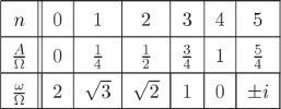
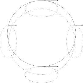
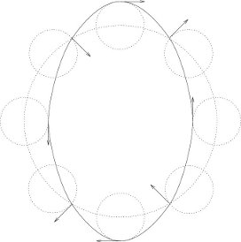
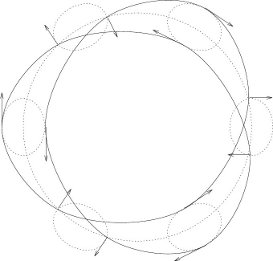
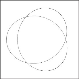
We can get some insight into the kinds of orbits produced by the epicyclic approximation by looking at a few examples. For some force laws we have integer ratios of epicyclic frequency to orbital frequency. In those cases we have closed orbits. For an inverse-square force law (n = 3) we get elliptical orbits with the center of the field at a focus of the ellipse. Figure 5.3 shows how an approximation to such an orbit can be constructed by superposition of the motion on an elliptical epicycle with the motion of the same frequency on a circle. If the force is proportional to the radius (n = 0) we get a two-dimensional harmonic oscillator. Here the epicyclic frequency is twice the orbital frequency. Figure 5.4 shows how this yields elliptical orbits that are centered on the source of the central force. An orbit is closed when ω/Ω is a rational fraction. If the force is proportional to the −3/4 power of the radius, the epicyclic frequency is 3/2 the orbital frequency. This yields the three-lobed pattern seen in figure 5.5. For other force laws the orbits predicted by this analysis are multi-lobed patterns produced by precessing approximate ellipses. Most of the cases have incommensurate epicyclic and orbital frequencies, leading to orbits that do not close in finite time.
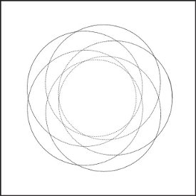
The epicyclic approximation gives a very good idea of what actual orbits look like. Figure 5.6, drawn by numerical integration of the orbit produced by integrating the original rectangular equations of motion for a particle in the field, shows the rosette-type picture characteristic of incommensurate epicyclic and orbital frequencies for an F = −r−2.3 force law.
We can directly compare a numerically integrated system with one of our epicyclic approximations. For example, the result of numerically integrating our F ∝ r−3/4 system is very similar to the picture we obtained by epicycles. (See figure 5.7 and compare it with figure 5.5.)
Exercise 5.11: Collapsing orbits
What exactly happens as the force law becomes steeper? Investigate this by sketching the contours of the Hamiltonian in r, pr space for various values of the force-law exponent, n. For what values of n are there stable circular orbits? In the case that there are no stable circular orbits, what happens to circular and other noncircular orbits? How are these results consistent with Liouville's theorem and the nonexistence of attractors in Hamiltonian systems?
5.4.5 Total Time Derivatives
The addition of a total time derivative to a Lagrangian leads to the same Lagrange equations. However, the two Lagrangians have different momenta, and they lead to different Hamilton's equations. Here we find out how to represent the corresponding canonical transformation with a generating function.
Let's restate the result about total time derivatives and Lagrangians from the first chapter. Consider some function G(t, q) of time and coordinates. We have shown that if L and L′ are related by
then the Lagrange equations of motion are the same. The generalized coordinates used in the two Lagrangians are the same, but the momenta conjugate to the coordinates are different. In the usual way, define
and
So we have
Evaluated on a trajectory, we have
This transformation is a special case of an F2-type transformation. Let
then the associated transformation is
Explicitly, the new Hamiltonian is
where we have used the fact that q = q′. The transformation is interesting in that the coordinate transformation is the identity transformation, but the new and old momenta are not the same, even in the case in which G has no explicit time dependence. Suppose we have a Hamiltonian of the form
then the transformed Hamiltonian is
We see that this transformation may be used to modify terms in the Hamiltonian that are linear in the momenta. Starting from H, the transformation introduces linear momentum terms; starting from H′, the transformation eliminates the linear terms.
Driven pendulum
We illustrate the use of this transformation with the driven pendulum. The Hamiltonian for the driven pendulum derived from the T − V Lagrangian (see section 1.6.2) is
where ys is the drive function. The Hamiltonian is rather messy, and includes a term that is linear in the angular momentum with a coefficient that depends on both the angular coordinate and the time. Let's see what happens if we apply our transformation to the problem to eliminate the linear term. We can identify the transformation function G by requiring that the linear term in momentum be killed:
The transformed momentum is
and the transformed Hamiltonian is
Dropping the last two terms, which do not affect the equations of motion, we find
So we have found, by a straightforward canonical transformation, a Hamiltonian for the driven pendulum with the rather simple form of a pendulum with gravitational acceleration that is modified by the acceleration of the pivot. It is, in fact, the Hamiltonian that corresponds to the alternative form of the Lagrangian for the driven pendulum that we found earlier by inspection (see equation 1.120). Here the derivation is by a simple canonical transformation, motivated by a desire to eliminate unwanted terms that are linear in the momentum.
Exercise 5.12: Construction of generating functions
Suppose that canonical transformations
are generated by two F1-type generating functions, F1a(t, q, q′) and F1b(t, q′, q″).
a. Show that the generating function for the inverse transformation of Ca is F1c(t, q′, q) = −F1a(t, q, q′).
b. Define a new kind of generating function,
Fx(t, q, q′, q″) = F1a(t, q, q′) + F1b(t, q′, q″).
We see that
p = ∂1Fx(t, q, q′, q″) = ∂1F1a(t, q, q′)
p″ = −∂3Fx(t, q, q′, q″) = −∂2F1b(t, q′, q″)
Show that ∂2Fx = 0, allowing a solution to eliminate q′.
c. Using the formulas for p and p″ above, and the result from part b, Show that Fx is an appropriate generating function for the composition transformation Ca ∘ Cb.
Exercise 5.13: Linear canonical transformations
We consider systems with two degrees of freedom and transformations for which the Hamiltonian transforms by composition.
a. Consider the linear canonical transformations that are generated by
Show that these transformations are just the point transformations, and that the corresponding F1 is zero.
b. Other linear canonical transformations can be generated by
Surely we can make even more generators by constructing F3- and F4-type transformations analogously. Are all of the linear canonical transformations obtainable in this way? If not, show one that cannot be so generated.
c. Can all linear canonical transformations be generated by compositions of transformations generated by the functions shown in parts a and b above?
d. How many independent parameters are necessary to specify all possible linear canonical transformations for systems with two degrees of freedom?
Exercise 5.14: Integral invariants
Consider the linear canonical transformation for a system with two degrees of freedom generated by the function
and the general parallelogram with a vertex at the origin and with adjacent sides starting at the origin and extending to the phase-space points (x1a, x2a, p1a, p2a) and (x1b, x2b, p1b, p2b).
a. Find the area of the given parallelogram and the area of the target parallelogram under the canonical transformation. Notice that the area of the parallelogram is not preserved.
b. Find the areas of the projections of the given parallelogram and the areas of the projections of the target under canonical transformation. Show that the sum of the areas of the projections on the action-like planes is preserved.
Exercise 5.15: Standard-map generating function
Find a generating function for the standard map (see exercise 5.8 on page 357).
5.5 Extended Phase Space
In this section we show that we can treat time as just another coordinate if we wish. Systems described by a time-dependent Hamiltonian may be recast in terms of a time-independent Hamiltonian with an extra degree of freedom. An advantage of this view is that what was a time-dependent canonical transformation can be treated as a time-independent transformation, where there are no additional conditions for adjusting the Hamiltonian.
Suppose that we have some system characterized by a time-dependent Hamiltonian, for example, a periodically driven pendulum. We may imagine that there is some extremely massive oscillator, unperturbed by the motion of the relatively massless pendulum, that produces the drive. Indeed, we may think of time itself as the coordinate of an infinitely massive particle moving uniformly and driving everything else. We often consider the rotation of the Earth as exactly such a stable time reference when performing short-time experiments in the laboratory.
More formally, consider a dynamical system with n degrees of freedom, whose behavior is described by a possibly time-dependent Lagrangian L with corresponding Hamiltonian H. We make a new dynamical system with n + 1 degrees of freedom by extending the generalized coordinates to include time and introducing a new independent variable. We also extend the generalized velocities to include a velocity for the time coordinate. In this new extended state space the coordinates are redundant, so there is a constraint relating the time coordinate to the new independent variable.
We relate the original dynamical system to the extended dynamical system as follows: Let q be a coordinate path. Let (qe, t) : τ ↦ (qe(τ), t(τ)) be a coordinate path in the extended system where τ is the new independent variable. Then qe = q ∘ t, or qe(τ) = q(t(τ)). Consequently, if v = Dq is the velocity along a path then ve(τ) = Dqe(τ) = Dq(t(τ)) · Dt(τ) = v(t(τ)) · vt(τ).
We can find a Lagrangian for the extended system by requiring that the value of the action be unchanged. Introduce the extended Lagrangian action
with
We have
The extended system is subject to a constraint that relates the time to the new independent variable. We assume the constraint is of the form φ(τ; qe, t; ve, vt) = t − f(τ) = 0. The constraint is a holonomic constraint involving the coordinates and time, so we can incorporate this constraint by augmenting the Lagrangian:24
The Lagrange equations of
The momenta conjugate to the coordinates are
So the extended momenta have the same values as the original momenta at the corresponding states. The momentum conjugate to the time coordinate is the negation of the energy plus vλ. The momentum conjugate to λ is the constraint, which must be zero.
Next we carry out the transformation to the corresponding Hamiltonian formulation. First, note that the Lagrangian Le is a homogeneous form of degree one in the velocities. Thus, by Euler's theorem,
The
So the Hamiltonian
We have used the fact that at corresponding states the momenta have the same values, so on paths pe = p ∘ t, and
The Hamiltonian
This extended Hamiltonian governs the evolution of the extended system, for arbitrary f.25
Hamilton's equations reduce to
The second equation gives the required relation between t and τ. The first and third equations are equivalent to Hamilton's equations in the original coordinates, as we can see by using qe = q ∘ t to rewrite them:
Using Dt(τ) = Df(τ) and dividing these factors out, we recover Hamilton's equations.26
Now consider the special case for which the time is the same as the independent variable: f(τ) = τ, Df(τ) = 1. In this case q = qe and p = pe. The extended Hamiltonian becomes
Hamilton's equation for t becomes Dt(τ) = 1, restating the constraint. Hamilton's equations for Dqe and Dpe are directly Hamilton's equations:
The extended Hamiltonian (5.274) does not depend on the independent variable, so it is a conserved quantity. Thus, up to an additive constant pt is equal to minus the energy. The Hamilton's equation for Dpt relates the change of the energy to ∂0H. Note that in the more general case, the momentum conjugate to the time is not the negation of the energy. This choice, t(τ) = τ, is useful for a number of applications.
The extension transformation is canonical in the sense that the two sets of equations of motion describe equivalent dynamics. However, the transformation is not symplectic; in fact, it does not even have the same number of input and output variables.
Exercise 5.16: Homogeneous extended Lagrangian
Verify that Le is homogeneous of degree one in the velocities.
Exercise 5.17: Lagrange equations
a. Verify that the Lagrange equations for qe are satisfied for exactly the same trajectories that satisfy the original Lagrange equations for q.
b. Verify that the Lagrange equation for t relates the rate of change of energy to ∂0L.
Exercise 5.18: Lorentz transformations
Investigate Lorentz transformations as point transformations in the extended phase space.
Restricted three-body problem
An example that shows the utility of reformulating a problem in the extended phase space is the restricted three-body problem: the motion of a low-mass particle subject to the gravitational attraction of two other massive bodies that move in some fixed orbit. The problem is an idealization of the situation where a body with very small mass moves in the presence of two bodies with much larger masses. Any effects of the smaller body on the larger bodies are neglected. In the simplest version, the motion of all three bodies is assumed to be in the same plane, and the orbits of the two massive bodies are circular.
The motion of the bodies with larger masses is not influenced by the small mass, so we model this situation as the small body moving in a time-varying field of the larger bodies undergoing a prescribed motion. This situation can be captured as a time-dependent Hamiltonian:
where r1(t) and r2(t) are the distances of the small body to the larger bodies, m is the mass of the small body, and m1 and m2 are the masses of the larger bodies. Note that r1(t) and r2(t) are quantities that depend both on the position of the small particle and the time-varying position of the massive particles.
The massive bodies are in circular orbits and maintain constant distance from the center of mass. Let a1 and a2 be the distances to the center of mass; then the distances satisfy m1a1 = m2a2. The angular frequency is
In polar coordinates, with the center of mass of the subsystem of massive particles at the origin and with r and θ describing the position of the low-mass particle, the positions of the two massive bodies are a2 = m1a/(m1+m2) with θ2 = Ωt, a1 = m2a/(m1+m2) with θ1 = Ωt + π. The distances to the point masses are
In polar coordinates, the Hamiltonian is
The Hamiltonian can be written in terms of some function f such that
The essential feature is that θ and t appear in the Hamiltonian only in the combination θ − Ωt.
One way to get rid of the time dependence is to choose a new set of variables with one coordinate equal to this combination θ − Ωt, by making a point transformation to a rotating coordinate system. We have shown that
with
is a canonical transformation. The new Hamiltonian, which is not the energy, is conserved because there is no explicit time dependence. It is a useful conserved quantity—the Jacobi constant.27
We can also eliminate the dependence on the independent time-like variable from the Hamiltonian for the restricted problem by going to the extended phase space, choosing t = τ. The Hamiltonian
is autonomous and is consequently a conserved quantity. Again, we see that θ and t occur only in the combination θ − Ωt, which suggests a point transformation to a new coordinate θ′ = θ − Ωt. This point transformation is independent of the new independent variable τ. The transformation is specified in equations (5.280–5.283), augmented by relations specifying how the time coordinate and its conjugate momentum are handled:
The new Hamiltonian is obtained by composing the old Hamiltonian with the transformation:
We recognize that the new Hamiltonian in the extended phase space, which has the same value as the original Hamiltonian in the extended phase space, is just the Jacobi constant plus
Exercise 5.19: Transformations in the extended phase space
In section 5.2.1 we found that time-dependent transformations for which the derivative of the coordinate–momentum part is symplectic are canonical only if the Hamiltonian is modified by adding a function K subject to certain constraints (equation 5.42). Show that the constraints on K follow from the symplectic condition in the extended phase space, using the choice t = τ.
5.5.1 Poincaré–Cartan Integral Invariant
The Poincaré invariant (section 5.3) is especially useful in the extended phase space with t = τ. In the extended phase space the extended Hamiltonian does not depend on the independent variable. In the extended phase space canonical transformations are symplectic and the Hamiltonian transforms by composition.
For the special choice of t = τ, equation (5.90) can be rephrased in an interesting way. Let E be the value of the Hamiltonian in the original unextended phase space. Using qn = t and pn = pt = −E, we can write
and
The relations (5.289) and (5.290) are two formulations of the Poincaré–Cartan integral invariant.
5.6 Reduced Phase Space
Suppose we have a system with n+1 degrees of freedom described by a time-independent Hamiltonian in a (2n + 2)-dimensional phase space. Here we can play the converse game: we can choose any generalized coordinate to play the role of “time” and the negation of its conjugate momentum to play the role of a new n-degree-of-freedom time-dependent Hamiltonian in a reduced phase space of 2n dimensions.
More precisely, let
and suppose we have a system described by a time-independent Hamiltonian
For each solution path there is a conserved quantity E. Let's choose a coordinate qn to be the time in a reduced phase space. We define the dynamical variables for the n-degree-of-freedom reduced phase space:
In the original phase space a coordinate such as qn maps time to a coordinate. In the formulation of the reduced phase space we will have to use the inverse function τ = (qn)−1 to map the coordinate to the time, giving the new coordinates in terms of the new time
and thus
We propose that a Hamiltonian in the reduced phase space is the negative of the inverse of f(q0, …, qn; p0, …, pn) = E with respect to the pn argument:
Note that in the reduced phase space we will have indices for the structured variables in the range 0 … n−1, whereas in the original phase space the indices are in the range 0 … n. We will show that Hr is an appropriate Hamiltonian for the given dynamical system in the reduced phase space. To compute Hamilton's equations we must expand the implicit definition of Hr. We define an auxiliary function
Note that by construction this function is identically a constant g = E. Thus all of its partial derivatives are zero:
where we have suppressed the arguments. Solving for partials of Hr, we get
Using these relations, we can deduce the Hamilton's equations in the reduced phase space from the Hamilton's equations in the original phase space:
Orbits in a central field
Consider planar motion in a central field. We have already seen this expressed in polar coordinates in equation (3.100):
There are two degrees of freedom and the Hamiltonian is time independent. Thus the energy, the value of the Hamiltonian, is conserved on realizable paths. Let's forget about time and reparameterize this system in terms of the orbital radius r.28 To do this we solve
for pr, obtaining
which is the Hamiltonian in the reduced phase space.
Hamilton's equations are now quite simple:
The momentum pφ is independent of r (as it was with t), so for any particular orbit we may define a constant angular momentum L. Thus our problem ends up as a simple quadrature:
To see the utility of this procedure, we continue our example with a definite potential energy—a gravitating point mass:
When we substitute this into equation (5.307) we obtain a mess that can be simplified to
Integrating this, we obtain another mess, which can be simplified and rearranged to obtain the following:
This can be recognized as the polar-coordinate form of the equation of a conic section with eccentricity e and parameter p:
where
In fact, if the orbit is an ellipse with semimajor axis a, we have
and so we can identify the role of energy and angular momentum in shaping the ellipse:
What we get from analysis in the reduced phase space is the geometry of the trajectory, but we lose the time-domain behavior. The reduction is often worth the price.
Although we have treated time in a special way so far, we have found that time is not special. It can be included in the coordinates to make a driven system autonomous. And it can be eliminated from any autonomous system in favor of any other coordinate. This leads to numerous strategies for simplifying problems, by removing time variation and then performing canonical transforms on the resulting conservative autonomous system to make a nice coordinate that we can then dump back into the role of time.
Generating functions in extended phase space
We can represent canonical transformations with mixed-variable generating functions. We can extend these to represent transformations in the extended phase space. Let F2 be a generating function with arguments (t, q, p′). Then, the corresponding
The relations between the coordinates and the momenta are the same as before. We also have
The first equation gives the relationship between the original Hamiltonians:
as required. Time-independent canonical transformations, where H′ = H ∘ CH, have symplectic qp part. The generating-function representation of a time-dependent transformation does not depend on the independent variable in the extended phase space. So, in extended phase space the qp part of the transformation, which includes the time and the momentum conjugate to time, is symplectic.
Exercise 5.20: Rotating coordinates in extended phase space
In the extended phase space the time is one of the coordinates. Carry out the transformation to rotating coordinates using an F2-type generating function in the extended phase space. Compare Hamiltonian (5.178) to the Hamiltonian obtained by composition with the transformation.
5.7 Summary
Canonical transformations can be used to reformulate a problem in coordinates that are easier to understand or that expose some symmetry of a problem.
In this chapter we have investigated different representations of a dynamical system. We have found that different representations will be equivalent if the coordinate–momentum part of the transformation has a symplectic derivative, and if the Hamiltonian transforms in a specified way. If the phase-space transformation is time independent, then the Hamiltonian transforms by composition with the phase-space transformation. The symplectic condition can be equivalently expressed in terms of the fundamental Poisson brackets. The Poisson bracket and the ω function are invariant under canonical transformations. The invariance of ω implies that the sum of the areas of the projections onto fundamental coordinate–momentum planes is preserved (Poincaré integral invariant) by canonical transformations.
A generating function is a real-valued function of the phase-space coordinates and time that represents a canonical transformation through its partial derivatives. We found that every canonical transformation can be represented by a generating function. The proof depends on the Poincaré integral invariant.
We can formulate an extended phase space in which time is treated as another coordinate. Time-dependent transformations are simple in the extended phase space. In the extended phase space the Poincaré integral invariant is the Poincaré–Cartan integral invariant. We can also reformulate a time-independent problem as a time-dependent problem with fewer degrees of freedom, with one of the original coordinates taking on the role of time; this is the reduced phase space.
5.8 Projects
Exercise 5.21: Hierarchical Jacobi coordinates
A Hamiltonian for the n-body problem is
with
and
where xi is the tuple of rectangular coordinates for body i and pi is the tuple of conjugate linear momenta for body i.
The potential energy of the system depends only on the relative positions of the bodies, so the relative motion decouples from the center of mass motion. In this problem we explore canonical transformations that achieve this decoupling.
a. Canonical heliocentric coordinates. The coordinates transform as follows:
where X is the center of mass of the system, and
for i > 0, the differences of the position of body i and the body with index 0 (which might be the Sun). Find the associated canonical momenta using an F2-type generating function. Show that the potential energy can be written solely in terms of the coordinates for i > 0. Show that the kinetic energy is not in the form of a sum of squares of momenta divided by mass constants.
b. Jacobi coordinates. The Jacobi coordinates isolate the center of mass motion, without spoiling the usual diagonal quadratic form of the kinetic energy. Define Xi to be the center of mass of the bodies with indices less than or equal to i:
The Jacobi coordinates are defined by
for 0 < i < n, and
The coordinates
for some constants
c. Hierarchical Jacobi coordinates. Define a “body” as a tuple of a mass and a rectangular position tuple. An n-body “system” is a tuple of n bodies: (b0, b1, …, bn−1). Define a “linking” transformation
The bodies in the new system are the same as the bodies in the old system
This is a transformation to relative coordinates and center of mass for bodies j and k. Extend this transformation to phase space and show that it preserves the form of the kinetic energy
Show that the transformation to Jacobi coordinates of part b is generated by a composition of linking transformations:
Interpret the coordinate transformation produced by such a succession of linking transformations; why do we call this a “linking” transformation? What requirement has to be satisfied for a composition of linking transformations to isolate the center of mass of the system (make it one of the coordinates)? Taking this constraint into account, find hierarchical Jacobi coordinates for a system with six bodies, arranged as two triple systems, each of which is a binary plus a third body. Verify that one of the coordinates is the center of mass of the system, and that the kinetic energy remains a sum of squares of the momenta divided by an appropriate mass constant.
1 Solving for p in terms of p′ involves multiplying equation (5.3) on the right by (∂1F(t, q′))−1. This inverse is the structure that when multiplying ∂1F(t, q′) on the right gives an identity structure. Structures representing linear transformations may be represented in terms of matrices. In this case, the matrix representation of the inverse structure is the inverse of the matrix representing the given structure.
2In chapter 1 the transformation C takes a local tuple in one coordinate system and gives a local tuple in another coordinate system. In this chapter CH is a phase-space transformation.
3The velocities and the momenta are dual geometric objects with respect to time-independent point transformations. The velocities are coordinates of a vector field on the configuration manifold, and the momenta are coordinates of a covector field on the configuration manifold. The invariance of the inner product pv under time-independent point transformations provides a motivation for our use of superscripts for velocity components and subscripts for momentum components.
4The procedure solve-linear-right multiplies its first argument by the inverse of its second argument on the right. So, if u = vM then v = uM−1; (solve-linear-right u M) produces v.
5Ds is not a derivative operator. It is not linear because the time component is a nonzero constant.
6Sometimes we use a center dot to indicate multiplication, to avoid the ambiguity of the use of juxtaposition to indicate both multiplication and function application. This is not to be interpreted as a vector dot product.
7Actually, for I = 0 the transform is not well defined and so it is not canonical for that value. This transformation is “locally canonical” in that it is canonical for nonzero values of I. We will ignore this essentially topological problem.
8Unlike Ds,
9The procedure zero-like produces a structure of zeros with the shape of its argument.
10This is just a rearrangement of the arguments of Rz: R(Ω)(t, q′) = Rz(Ωt)(q′).
11For each linear transformation T : A → A of incremental phase-space states there is a unique linear transformation
12The procedure compatible-shape takes any structure and produces another structure that is guaranteed to multiply with the given structure to produce a numerical quantity. For example, the shape of DH(s) is a compatible shape to the shape of s: if they are multiplied the result is a numerical quantity. This is the s⋆ that appears in equation (5.48).
13The procedure transpose is simply defined for traditional matrices, but because structures that specify linear transformations may have arbitrary substructure, the procedure needs to be supplied with a template that specifies this structure. So the procedure transpose takes two arguments: (transpose ms rs), where ms is the structure to be transposed and the template rs is a structure that is appropriate for multiplication with ms on the right.
14Actually, this is more interesting: we allow transformations that arbitrarily distort time, as tau is an arbitrary literal function. The canonical condition is concerned only with the possibly time-dependent transformation of coordinates and momenta.
15The qp submatrix of a square matrix of dimension 2n + 1 is the 2n-dimensional matrix obtained by deleting the first row and the first column of the given matrix. This can be computed by:
(define (qp-submatrix m)
(m:submatrix m 1 (m:num-rows m) 1 (m:num-cols m)))16The procedure D-as-matrix is defined as:
(define ((D-as-matrix F) s)
(s->m (compatible-shape (F s)) ((D F) s) s)))17The qi, pi plane is the ith canonical plane in these phase-space variables.
18The structure ∂2∂1F1 is a down of downs, so it is compatible for contraction with an up on either side. But it is not symmetrical, so the associations must be specified. To solve this problem we use index notation (ugh!).
So we use indices to select particular components of structured objects. If an index symbol appears both as a superscript and as a subscript in an expression, the value of the expression is the sum over all possible values of the index symbol of the designated components (Einstein summation convention). Thus, for example, if
19A structure is nonsingular if the determinant of the matrix representation of the structure is nonzero.
20Point transformations are not in this class: we cannot solve for the momenta in terms of the positions for point transformations, because for a point transformation the primed and unprimed coordinates can be deduced from each other, so there is not enough information in the coordinates to deduce the momenta.
21Let F be defined as the path-independent line integral
then ∂iF(x) = fi(x).
22There may be some singular cases and topological problems that prevent this from being rigorously true.
23The various generating functions are traditionally known by the names F1, F2, F3, and F4. Please don't blame us.
24We augment the Lagrangian with the total time derivative of the constraint so that the Legendre transform will be well defined.
25Once we have made this reduction, taking pλ to be zero, we can no longer perform a Legendre transform back to the extended Lagrangian system; we cannot solve for pt in terms of vt. However, the Legendre transform in the extended system from
26If f is strictly increasing then Df is never zero.
27Actually, the traditional Jacobi constant is C = −2H′.
28We could have chosen to reparameterize in terms of φ, but then both pr and r would occur in the resulting time-independent Hamiltonian. The path we have chosen takes advantage of the fact that φ does not appear in our Hamiltonian, so pφ is a constant of the motion. This structure suggests that to solve this kind of problem we need to look ahead, as in playing chess.