6Canonical Evolution
What, then, is time? I know well enough what it is, provided that nobody asks me; but if I am asked what it is and try to explain, I am baffled. All the same I can confidently say that I know that if nothing passed, there would be no past time; if nothing were going to happen, there would be no future time; and if nothing were there would be no present time.
Augustine of Hippo, from Confessions, Book XI, Section 14. Translation by R.S. Pine-Coffin, 1961.
Time evolution generates a canonical transformation: if we consider all possible initial states of a Hamiltonian system and follow all the trajectories for the same time interval, then the map from the initial state to the final state of each trajectory is a canonical transformation. Hamilton–Jacobi theory gives a mixed-variable generating function that generates this time-evolution transformation. For the few integrable systems for which we can solve the Hamilton–Jacobi equation this transformation gets us action-angle coordinates, which form a starting point to study perturbations.
6.1 Hamilton–Jacobi Equation
If we could find a canonical transformation so that the transformed Hamiltonian was identically zero, then by Hamilton's equations the new coordinates and momenta would be constants. All of the time variation of the solution would be captured in the canonical transformation, and there would be nothing more to the solution. A mixed-variable generating function that does this job satisfies a partial differential equation called the Hamilton–Jacobi equation. In most cases, a Hamilton–Jacobi equation cannot be solved explicitly. When it can be solved, however, a Hamilton–Jacobi equation provides a means of reducing a problem to a useful simple form.
Recall the relations satisfied by an F2-type generating function:
If we require the new Hamiltonian to be zero, then F2 must satisfy the equation
So the solution of the problem is “reduced” to the problem of solving an n-dimensional partial differential equation for F2 with unspecified new (constant) momenta p′. This is a Hamilton–Jacobi equation, and in some cases we can solve it.
We can also attempt a somewhat less drastic method of solution. Rather than try to find an F2 that makes the new Hamiltonian identically zero, we can seek an F2-shaped function W that gives a new Hamiltonian that is solely a function of the new momenta. A system described by this form of Hamiltonian is also easy to solve. So if we set
and are able to solve for W, then the problem is essentially solved. In this case, the primed momenta are all constant and the primed positions are linear in time. This is an alternate form of the Hamilton–Jacobi equation.
These forms are related. Suppose that we have a W that satisfies the second form of the Hamilton–Jacobi equation (6.5). Then the F2 constructed from W
satisfies the first form of the Hamilton–Jacobi equation (6.4). Furthermore,
so the primed momenta are the same in the two formulations. But
so we see that the primed coordinates differ by a term that is linear in time—both
Note that if H is time independent then we can often find a time-independent W that does the job. For time-independent W the Hamilton–Jacobi equation simplifies to
The corresponding F2 is then linear in time. Notice that an implicit requirement is that the energy can be written as a function of the new momenta alone. This excludes the possibility that the transformed phase-space coordinates q′ and p′ are simply initial conditions for q and p.
It turns out that there is flexibility in the choice of the function E. With an appropriate choice the phase-space coordinates obtained through the transformation generated by W are action-angle coordinates.
Exercise 6.1: Hamilton–Jacobi with F1
We have used an F2-type generating function to carry out the Hamilton–Jacobi transformations. Carry out the equivalent transformations with an F1-type generating function. Find the equations corresponding to equations (6.4), (6.5), and (6.9).
6.1.1 Harmonic Oscillator
Consider the familiar time-independent Hamiltonian
We form the Hamilton–Jacobi equation for this problem:
Using F2(t, x, p′) = W (t, x, p′) − E(p′)t, we find
Writing this out explicitly yields
and solving for ∂1W gives
Integrating gives the desired W:
We can use either W or the corresponding F2 as the generating function. First, take W to be the generating function. We obtain the coordinate transformation by differentiating:
and then integrating to get
with some integration constant C(p′). Inverting this, we get the unprimed coordinate in terms of the primed coordinate and momentum:
The new Hamiltonian H′ depends only on the momentum:
The equations of motion are just
with solution
for initial conditions
where the angular frequency is
We can also use F2 = W − Et as the generating function. The new Hamiltonian is zero, so both x′ and p′ are constant, but the relationship between the old and new variables is
Plugging in the solution
It is interesting to note that the solution depends upon the constants E(p′) and DE(p′), but otherwise the motion is not dependent in any essential way on what the function E actually is. The momentum p is constant and the values of the constants are set by the initial conditions. Given a particular function E, the initial conditions determine p′, but the solution can be obtained without further specifying the E function.
If we choose particular functions E we can get particular canonical transformations. For example, a convenient choice is simply
for some constant α that will be chosen later. We find
So we see that a convenient choice is
with
The solution is just
The two transformation equations (6.26) and (6.28) are what we have called the polar-canonical transformation (equation 5.29). We have already shown that this transformation is canonical and that it solves the harmonic oscillator, but it was not derived. Here we have derived this transformation as a particular case of the solution of the Hamilton–Jacobi equation.
We can also explore other choices for the E function. For example, we could choose
Following the same steps as before, we find
So a convenient choice is again α = ω, leaving
with β = (km)1/4. By construction, this transformation is also canonical and also brings the harmonic oscillator problem into an easily solvable form:
The harmonic oscillator Hamiltonian has been transformed to what looks a lot like the Hamiltonian for a free particle. This is very interesting. Notice that whereas Hamiltonian (6.27) does not have a well defined Legendre transform to an equivalent Lagrangian, the “free particle” harmonic oscillator has a well defined Legendre transform:
Of course, there may be additional properties that make one choice more useful than others for particular applications.
Exercise 6.2: Pendulum
Formulate and solve a Hamilton–Jacobi equation for the pendulum; investigate both the circulating and oscillating regions of phase space. (Note: This is a long story and requires some knowledge of elliptic functions.)
6.1.2 Hamilton–Jacobi Solution of the Kepler Problem
We can use the Hamilton–Jacobi equation to find canonical coordinates that solve the Kepler problem. This is an essential first step in doing perturbation theory for orbital problems.
In rectangular coordinates (x, y, z), the Kepler Hamiltonian is
where r2 = x2 + y2 + z2 and
We try a generating function of the form
This is a partial differential equation in the three partial derivatives of W. We stare at it a while and give up.
Next we try converting to spherical coordinates. This is motivated by the fact that the potential energy depends only on r. The Hamiltonian in spherical coordinates (r, θ, φ), where θ is the colatitude and φ is the longitude, is
The Hamilton–Jacobi equation is
We can solve this Hamilton–Jacobi equation by successively isolating the dependence on the various variables. Looking first at the φ dependence, we see that, outside of W, φ appears only in one partial derivative. If we write
then
Any function of the
We can eliminate the θ dependence if we choose
and require that Θ be a solution to
We are free to choose the right-hand side to be any function of the new momenta. This choice reflects the fact that the left-hand side is non-negative. It turns out that
The remaining equation that determines R is
which also can be solved by quadrature.
Altogether the solution of the Hamilton–Jacobi equation reads
It is interesting that our solution to the Hamilton–Jacobi partial differential equation is of the form
Thus we have a separation-of-variables technique that involves writing the solution as a sum of functions of the individual variables. This might be contrasted with the separation-of-variables technique encountered in elementary quantum mechanics and classical electrodynamics, which uses products of functions of individual variables.
The coordinates q′ = (q′0, q′1, q′2) conjugate to the momenta
We are still free to choose the functional form of E. A convenient (and conventional) choice is
With this choice the momentum
The Hamiltonian for the Kepler problem is reduced to
Thus
where
The canonical phase-space coordinates can be written in terms of the parameters that specify an orbit. We merely summarize the results; for further explanation see [36] or [38].
Assume we have a bound orbit with semimajor axis a, eccentricity e, inclination i, longitude of ascending node Ω, argument of pericenter ω, and mean anomaly M. The three canonical momenta are
6.1.3 F2 and the Lagrangian
The solution to the Hamilton–Jacobi equation, the mixed-variable generating function that generates time evolution, is related to the action used in the variational principle. In particular, the time derivative of the generating function along realizable paths has the same value as the Lagrangian.
Let
Using the Hamilton–Jacobi equation (6.4), this becomes
Now, using equation (6.2), we get
But
On realizable paths we have Dp′(t) = 0, so along realizable paths the time derivative of F2 is the same as the Lagrangian along the path. The time integral of the Lagrangian along any path is the action along that path. This means that, up to an additive term that is constant on realizable paths but may be a function of the transformed phase-space coordinates q′ and p′, the F2 that solves the Hamilton–Jacobi equation has the same value as the Lagrangian action for realizable paths.
The same conclusion follows for the Hamilton–Jacobi equation formulated in terms of F1. Up to an additive term that is constant on realizable paths but may be a function of the transformed phase-space coordinates q′ and p′, the F1 that solves the corresponding Hamilton–Jacobi equation has the same value as the Lagrangian action for realizable paths.
Recall that a transformation given by an F2-type generating function is also given by an F1-type generating function related to it by a Legendre transform (see equation 5.142):
provided the transformations are nonsingular. In this case, both q′ and p′ are constant on realizable paths, so the additive constants that make F1 and F2 equal to the Lagrangian action differ by q′p′.
Exercise 6.3: Harmonic oscillator
Let's check this for the harmonic oscillator (of course).
a. Finish the integral (6.15):
Write the result in terms of the amplitude
b. Check that this generating function gives the transformation
which is the same as equation (6.17) for a particular choice of the integration constant. The other part of the transformation is
with the same definition of A as before.
c. Compute the time derivative of the associated F2 along realizable paths (Dp′(t) = 0), and compare it to the Lagrangian along realizable paths.
6.1.4 The Action Generates Time Evolution
We define the function
For variations η that are not necessarily zero at the end times and for realizable paths q, the variation of the action is
Alternatively, the variation of S[q] in equation (6.55) gives
Comparing equations (6.56) and (6.57) and using the fact that the variation η is arbitrary, we find
The partial derivatives of
This looks a bit like the F1-type generating function relations, but here there are two times. Solving equations (6.59) for q2 and p2 as functions of t2 and the initial state t1, q1, p1, we get the time evolution of the system in terms of
If we vary the lower limit of the action integral we get
Using equation (6.55), and given a realizable path q such that q(t1) = q1 and q(t2) = q2, we get the partial derivatives with respect to the time slots:
Rearranging the terms of equation (6.61) and using equation (6.60) we get
and similarly
These are a pair of Hamilton–Jacobi equations, computed at the endpoints of the path.
The function
The generating function for the composition is the difference of the generating functions for each step:
with the condition
which allows us to eliminate q′ in terms of t1, q1, t2, and q2. So we can write
Exercise 6.4: Uniform acceleration
a. Compute the Lagrangian action, as a function of the endpoints and times, for a uniformly accelerated particle. Use this to construct the canonical transformation for time evolution from a given initial state.
b. Solve the Hamilton–Jacobi equation for the uniformly accelerated particle, obtaining the F1 that makes the transformed Hamiltonian zero. Show that the Lagrangian action can be expressed as a difference of two applications of this F1.
6.2 Time Evolution is Canonical
We use time evolution to generate a transformation
that is obtained in the following way. Let
or, equivalently,
Notice that
Given a state (t′, q′, p′), we find the phase-space path σ emanating from this state as an initial condition, satisfying
The value (t, q, p) of
Time evolution is canonical if the transformation
Let ζ′ be an increment with zero time component of the state (t′, q′, p′). The linearized increment in the value of
be variations of the state path
The symplectic requirement is
This must be true for arbitrary Δ, so it is satisfied if the following quantity is constant:
We compute the derivative:
With Hamilton's equations, the variations satisfy
Substituting these into DA and collecting terms, we find3
We conclude that time evolution generates a phase-space transformation with symplectic derivative.
To make a canonical transformation we must specify how the Hamiltonian transforms. The same Hamiltonian describes the evolution of a state and a time-advanced state because the latter is just another state. Thus the transformed Hamiltonian is the same as the original Hamiltonian.
Liouville's theorem, again
We deduced that volumes in phase space are preserved by time evolution by showing that the divergence of the phase flow is zero, using the equations of motion (see section 3.8). We can also show that volumes in phase space are preserved by the evolution using the fact that time evolution is a canonical transformation.
We have shown that phase-space volume is preserved for sym-plectic transformations. Now we have shown that the transformation generated by time evolution is a symplectic transformation. Therefore, the transformation generated by time evolution preserves phase-space volume. This is an alternate proof of Liouville's theorem.
Another time-evolution transformation
There is another canonical transformation that can be constructed from time evolution. We define the transformation
where SΔ(a, b, c) = (a + Δ, b, c) shifts the time of a phase-space state.4 More explicitly, given a state (t, q′, p′), we evolve the state that is obtained by subtracting Δ from t; that is, we take the state (t − Δ, q′, p′) as an initial state for evolution by Hamilton's equations. The state path σ satisfies
The output of the transformation is the state
The transformation satisfies
The arguments of
Why is this a good idea? Our usual canonical transformations do not change the time component. The
The
or
Notice that if H is time independent then
Assume we have a procedure C such that ((C delta-t) state) implements a time-evolution transformation
(define ((C->Cp C) delta-t)
  (compose (C delta-t) (shift-t (- delta-t))))
where shift-t implements SΔ:
(define ((shift-t delta-t) state)
  (up
    (+ (time state) delta-t)
    (coordinate state)
    (momentum state)))
To complete the canonical transformation we have a procedure that transforms the Hamiltonian:
(define ((H->Hp delta-t) H)
  (compose H (shift-t (- delta-t))))
So both
Exercise 6.5: Verification
The condition (5.20) that Hamilton's equations are preserved for
and the condition that Hamilton's equations are preserved for
Verify that these conditions are satisfied.
Exercise 6.6: Driven harmonic oscillator
We can use the simple driven harmonic oscillator to illustrate that time evolution yields a symplectic transformation that can be extended to be canonical in two ways. We use the driven harmonic oscillator because its solution can be compactly expressed in explicit form.
Suppose that we have a harmonic oscillator with natural frequency ω0 driven by a periodic sinusoidal drive of frequency ω and amplitude α. The Hamiltonian we will consider is
The general solution for a given initial state (t0, q0, p0) evolved for a time Δ is
where
a. Fill in the details of the procedure
(define (((C* alpha omega omega0) delta-t) state)
  ... )
that implements the time-evolution transformation of the driven harmonic oscillator. Let C be (C* alpha omega omega0).
b. In terms of C*, the general solution emanating from a given state is
(define (((solution alpha omega omega0) state0) t)
  (((C* alpha omega omega0) (- t (time state0))) state0))
Check that the implementation of C* is correct by using it to construct the solution and verifying that the solution satisfies Hamilton's equations. Further check the solution by comparing to numerical integration.
c. We know that for any phase-space state function F the rate of change of that function along a solution path σ is
Show, by writing a short program to test it, that this is true of the function implemented by (C delta) for the driven oscillator. Why is this interesting?
d. Use the procedure symplectic-transform? to show that both C and Cp are symplectic.
e. Use the procedure canonical? to verify that both C and Cp are canonical with the appropriate transformed Hamiltonian.
6.2.1 Another View of Time Evolution
We can also show that time evolution generates canonical transformations using the Poincaré–Cartan integral invariant.
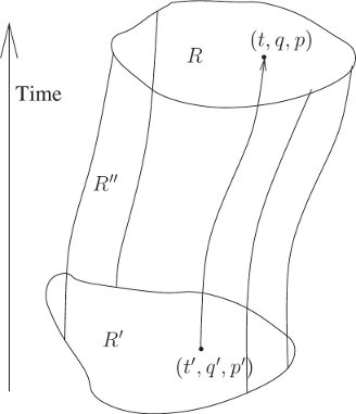
Consider a two-dimensional region of phase-space coordinates, R′, at some particular time t′ (see figure 6.1). Let R be the image of this region at time t under time evolution for a time interval of Δ. The time evolution is governed by a Hamiltonian H. Let
In the extended phase space we see that the evolution sweeps out a cylindrical volume with endcaps R′ and R, each at a fixed time. Let R″ be the two-dimensional region swept out by the trajectories that map the boundary of region R′ to the boundary of region R. The regions R, R′, and R″ together form the boundary of a volume of phase-state space.
The Poincaré–Cartan integral invariant on the whole boundary is zero.6 Thus
where the n index indicates the t, pt canonical plane. The second term is negative, because in the extended phase space we take the area to be positive if the normal to the surface is outward pointing.
We will show that the Poincaré–Cartan integral invariant for a region of phase space that is generated by time evolution is zero:
This will allow us to conclude
The areas of the projection of R and R′ on the t, pt plane are zero because R and R′ are at constant times, so for these regions the Poincaré–Cartan integral invariant is the same as the Poincaré integral invariant. Thus
We are left with showing that the Poincaré–Cartan integral invariant for the region R″ is zero. This will be zero if the contribution from any small piece of R″ is zero. We will show this by showing that the ω form (see equation 5.70) on a small parallelogram in this region is zero. Let (0; q, t; p, pt) be a vertex of this parallelogram. The parallelogram is specified by two edges ζ1 and ζ2 emanating from this vertex. For edge ζ1 of the parallelogram, we take a constant-time phase-space increment with length Δq and Δp in the q and p directions. The first-order change in the Hamiltonian that corresponds to these changes is
for constant time Δt = 0. The increment Δpt is the negative of ΔH. So the extended phase-space increment is
The edge ζ2 is obtained by time evolution of the vertex for a time interval Δt. Using Hamilton's equations, we obtain
The ω form applied to these incremental states that form the edges of this parallelogram gives the area of the parallelogram:
So we may conclude that the integral of this expression over the entire surface of the tube of trajectories is also zero. Thus the Poincaré–Cartan integral invariant is zero for any region that is generated by time evolution.
Having proven that the trajectory tube provides no contribution, we have shown that the Poincaré integral invariant of the two endcaps is the same. This proves that time evolution generates a symplectic qp transformation.
Area preservation of surfaces of section
We can use the Poincaré–Cartan invariant to prove that for autonomous two-degree-of-freedom systems, surfaces of section (constructed appropriately) preserve area.
To show this we consider a surface of section for one coordinate (say q2) equal to zero. We construct the section by accumulating the (q1, p1) pairs. We assume that all initial conditions have the same energy. We compute the sum of the areas of canonical projections in the extended phase space again. Because all initial conditions have the same q2 = 0 there is no area on the q2, p2 plane, and because all the trajectories have the same value of the Hamiltonian the area of the projection on the t, pt plane is also zero. So the sum of areas of the projections is just the area of the region on the surface of section. Now let each point on the surface of section evolve to the next section crossing. For each point on the section this may take a different amount of time. Compute the sum of the areas again for the mapped region. Again, all points of the mapped region have the same q2, so the area on the q2, p2 plane is zero, and they continue to have the same energy, so the area on the t, pt plane is zero. So the area of the mapped region is again just the area on the surface of section, the q1, p1 plane. Time evolution preserves the sum of areas, so the area on the surface of section is the same as the mapped area.
Thus surfaces of section preserve area provided that the section points are entirely on a canonical plane. For example, to make the Hénon–Heiles surfaces of section (see section 3.6.3) we plotted py versus y when x = 0 with px ≥ 0. So for all section points the x coordinate has the fixed value 0, the trajectories all have the same energy, and the points accumulated are entirely in the y, py canonical plane. So the Hénon–Heiles surfaces of section preserve area.
6.2.2 Yet Another View of Time Evolution
We can show directly from the action principle that time evolution generates a symplectic transformation.
Recall that the Lagrangian action S is
We computed the variation of the action in deriving the Lagrange equations. The variation is (see equation 1.33)
rewritten in terms of the Euler–Lagrange operator
Recall that p and η are structures, and the product implies a sum of products of components.
Consider a continuous family of realizable paths; the path for parameter s is
be the value of the action from t1 to t2 for path
Because
where
where
In conventional notation the latter line integral is written
where
For a loop family of paths (such that
which is the line-integral version of the integral invariants.
In terms of area integrals, using Stokes's theorem, this is
where
6.3 Lie Transforms
The evolution of a system under any Hamiltonian generates a continuous family of canonical transformations. To study the behavior of some system governed by a Hamiltonian H, it is sometimes appropriate to use a canonical transformation generated by evolution governed by another Hamiltonian-like function W on the same phase space. Such a canonical transformation is called a Lie transform.
The functions H and W are both Hamiltonian-shaped functions defined on the same phase space. Time evolution for an interval Δ governed by H is a canonical transformation
The independent variable in the H evolution is time, and the independent variable in the W evolution is an arbitrary parameter of the canonical transformation. We chose

Figure 6.2 shows how a Lie transform is used to transform a trajectory. We can see from the diagram that the canonical transformations obey the relation
For generators W that do not depend on the independent variable, the resulting canonical transformation
We will use only Lie transforms that have generators that do not depend on the independent variable.
Lie transforms of functions
The value of a phase-space function F changes if its arguments change. We define the function
We say that
In particular, the Lie transform advances the coordinate and momentum selector functions Q = I1 and P = I2:
So we may restate equation (6.107) as
More generally, Lie transforms descend into compositions:
A corollary of the fact that Lie transforms descend into compositions is:
where I is the phase-space identity function: I(t, q, p) = (t, q, p). So the order of application of the operators is reversed from the order of composition of the functions that result from applying the operators.
In terms of
We can also say
Note that
The identity I is
We can define the inverse function
with the property
Simple Lie transforms
For example, suppose we are studying a system for which a rotation would be a helpful transformation. To concoct such a transformation we note that we intend a configuration coordinate to increase uniformly with a given rate. In this case we want an angle to be incremented. The Hamiltonian that consists solely of the momentum conjugate to that configuration coordinate always does the job. So the angular momentum is an appropriate generator for rotations.
The analysis is simple if we use polar coordinates r, θ with conjugate momenta pr, pθ. The generator W is just:
The family of transformations satisfies Hamilton's equations:
The only variable that appears in W is pθ, so θ is the only variable that varies as ϵ is varied. In fact, the family of canonical transformations is
So angular momentum is the generator of a canonical rotation.
The example is simple, but it illustrates one important feature of Lie transformations—they give one set of variables entirely in terms of the other set of variables. This should be contrasted with the mixed-variable generating function transformations, which always give a mixture of old and new variables in terms of a mixture of new and old variables, and thus require an inversion to get one set of variables in terms of the other set of variables. This inverse can be written in closed form only for special cases. In general, there is considerable advantage in using a transformation rule that generates explicit transformations from the start. The Lie transformations are always explicit in the sense that they give one set of variables in terms of the other, but for there to be explicit expressions the evolution governed by the generator must be solvable.
Let's consider another example. This time consider a three-degree-of-freedom problem in rectangular coordinates, and take the generator of the transformation to be the z component of the angular momentum:
The evolution equations are
We notice that z and pz are unchanged, and that the equations governing the evolution of x and y decouple from those of px and py. Each of these pairs of equations represents simple harmonic motion, as can be seen by writing them as second-order systems. The solutions are
So we see that again a component of the angular momentum generates a canonical rotation. There was nothing special about our choice of axes, so we can deduce that the component of angular momentum about any axis generates rotations about that axis.
Example
Suppose we have a system governed by the Hamiltonian
Hamilton's equations couple the motion of x and y:
We can decouple the system by performing a coordinate rotation by π/4. This is generated by
which is similar to the generator for the coordinate rotation above but without the z degree of freedom. Evolving (τ; x, y; px, py) by W for an interval of π/4 gives a canonical rotation:
Composing the Hamiltonian H with this time-independent transformation gives the new Hamiltonian
which is a Hamiltonian for two uncoupled harmonic oscillators. So the original coupled problem has been transformed by a Lie transform to a new form for which the solution is easy.
6.4 Lie Series
A convenient way to compute a Lie transform is to approximate it with a series. We develop this technique by extending the idea of a Taylor series.
Taylor's theorem gives us a way of approximating the value of a nice enough function at a point near to a point where the value is known. If we know f and all of its derivatives at t then we can get the value of f(t + ϵ), for small enough ϵ, as follows:
We recall that the power series for the exponential function is
This suggests that we can formally construct a Taylor-series operator as the exponential of a differential operator10
and write
We have to be a bit careful here: (ϵD)2 = ϵDϵD. We can turn it into ϵ2D2 only because ϵ is a scalar constant, which commutes with every differential operator. But with this caveat in mind we can define the differential operator
Before going on, it is interesting to compute with these a bit. In the code transcripts that follow we develop the series by exponentiation. We can examine the series incrementally by looking at successive elements of the (infinite) sequence of terms of the series. The procedure series:for-each is an incremental traverser that applies its first argument to successive elements of the series given as its second argument. The third argument (when given) specifies the number of terms to be traversed. In each of the following transcripts we print simplified expressions for the successive terms.
The first thing to look at is the general Taylor expansion for an unknown literal function, expanded around t, with increment ϵ. Understanding what we see in this simple problem will help us understand more complex problems later.
(series:for-each print-expression
                 (((exp (* 'epsilon D))
                   (literal-function 'f))
                  't)
6)(f t)
(* ((D f) t) epsilon)
(* 1/2 (((expt D 2) f) t) (expt epsilon 2))
(* 1/6 (((expt D 3) f) t) (expt epsilon 3))
(* 1/24 (((expt D 4) f) t) (expt epsilon 4))
(* 1/120 (((expt D 5) f) t) (expt epsilon 5))
...We can also look at the expansions of particular functions that we recognize, such as the expansion of sin around 0.
(series:for-each print-expression
                 (((exp (* 'epsilon D)) sin) 0)
                 6)
0
epsilon
0
(* -1/6 (expt epsilon 3))
0
(* 1/120 (expt epsilon 5))
...It is often instructive to expand functions we usually don't remember, such as
(series:for-each print-expression
                 (((exp (* 'epsilon D))
                   (lambda (x) (sqrt (+ x 1))))
                  0)
                 6)
1
(* 1/2 epsilon)
(* -1/8 (expt epsilon 2))
(* 1/16 (expt epsilon 3))
(* -5/128 (expt epsilon 4))
(* 7/256 (expt epsilon 5))
...Exercise 6.7: Binomial series
Develop the binomial expansion of (1 + x)n as a Taylor expansion. Of course, it must be the case that for n a positive integer all of the coefficients except for the first n + 1 are zero. However, in the general case, for symbolic n, the coefficients are rather complicated polynomials in n. For example, you will find that the eighth term is
(+ (* 1/5040 (expt n 7))
   (* -1/240 (expt n 6))
   (* 5/144 (expt n 5))
   (* -7/48 (expt n 4))
   (* 29/90 (expt n 3))
   (* -7/20 (expt n 2))
   (* 1/7 n))
These terms must evaluate to the entries in Pascal's triangle. In particular, this polynomial must be zero for n < 7. How is this arranged?
Dynamics
Now, to play this game with dynamical functions we want to provide a derivative-like operator that we can exponentiate, which will give us the time-advance operator. The key idea is to write the derivative of the function in terms of the Poisson bracket. Equation (3.80) shows how to do this in general:
We define the operator DH by
so
and iterates of this operator can be used to compute higher-order derivatives:
We can express the advance of the path function f = F ∘ σ for an interval ϵ with respect to H as a power series in the derivative operator DH applied to the phase-space function F and then composed with the path:
Indeed, we can implement the time-advance operator Eϵ,H with this series, when it converges.
Exercise 6.8: Iterated derivatives
Show that equation (6.138) is correct.
Exercise 6.9: Lagrangian analog
Compare DH with the total time derivative operator. Recall that
abstracts the derivative of a function of a path through state space to a function of the derivatives of the path. Define another derivative operator DL, analogous to DH, that would give the time derivative of functions along Lagrangian state paths that are solutions of Lagrange's equations for a given Lagrangian. How might this be useful?
For time-independent Hamiltonian H and time-independent state function F, we can simplify the computation of the advance of F. In this case we define the Lie derivative operator LH such that
which reads “the Lie derivative of F with respect to H.”11 So
and for time-independent F
We can iterate this process to compute higher derivatives. So
and successively higher-order Poisson brackets of F with H give successively higher-order derivatives when evaluated on the trajectory.
Let f = F ∘ σ. We have
Thus we can rewrite the advance of the path function f for an interval ϵ with respect to H as a power series in the Lie derivative operator applied to the phase-space function F and then composed with the path:
We can implement the time-advance operator
We have shown that time evolution is canonical, so the series above are formal representations of canonical transformations as power series in the time. These series may not converge, even if the evolution governed by the Hamiltonian H is well defined.
Computing Lie series
We can use the Lie transform as a computational tool to examine the local evolution of dynamical systems. We define the Lie derivative of F as a derivative-like operator relative to the given Hamiltonian function, H:12
(define ((Lie-derivative H) F)
  (Poisson-bracket F H))
We also define a procedure to implement the Lie transform:13
(define (Lie-transform H t)
  (exp (* t (Lie-derivative H))))
Let's start by examining the beginning of the Lie series for the position of a simple harmonic oscillator of mass m and spring constant k. We can implement the Hamiltonian as
(define ((H-harmonic m k) state)
  (+ (/ (square (momentum state)) (* 2 m))
     (* 1/2 k (square (coordinate state)))))
We make the Lie transform (series) by passing the Lie-transform operator an appropriate Hamiltonian function and an interval to evolve for. The resulting operator is then given the coordinate procedure, which selects the position coordinates from the phase-space state. The Lie transform operator returns a procedure that, when given a phase-space state composed of a dummy time, a position x0, and a momentum p0, returns the position resulting from advancing that state by the interval dt.
(series:for-each print-expression
                 (((Lie-transform (H-harmonic 'm 'k) 'dt)
                   coordinate)
                  (up 0 'x0 'p0))
                 6)
x0
(/ (* dt p0) m)
(/ (* -1/2 (expt dt 2) k x0) m)
(/ (* -1/6 (expt dt 3) k p0) (expt m 2))
(/ (* 1/24 (expt dt 4) (expt k 2) x0) (expt m 2))
(/ (* 1/120 (expt dt 5) (expt k 2) p0) (expt m 3))
...We should recognize the terms of this series. We start with the initial position x0. The first-order correction (p0/m)dt is due to the initial velocity. Next we find an acceleration term (−kx0/2m)dt2 due to the restoring force of the spring at the initial position.
The Lie transform is just as appropriate for showing us how the momentum evolves over the interval:
(series:for-each print-expression
                 (((Lie-transform (H-harmonic 'm 'k) 'dt)
                   momentum)
                  (up 0 'x0 'p0))
                 6)
p0
(* -1 dt k x0)
(/ (* -1/2 (expt dt 2) k p0) m)
(/ (* 1/6 (expt dt 3) (expt k 2) x0) m)
(/ (* 1/24 (expt dt 4) (expt k 2) p0) (expt m 2))
(/ (* -1/120 (expt dt 5) (expt k 3) x0) (expt m 2))
...In this series we see how the initial momentum p0 is corrected by the effect of the restoring force −kx0dt, etc.
What is a bit more fun is to see how a more complex phase-space function is treated by the Lie series expansion. In the experiment below we examine the Lie series developed by advancing the harmonic-oscillator Hamiltonian, by means of the transform generated by the same harmonic-oscillator Hamiltonian:
(series:for-each print-expression
                 (((Lie-transform (H-harmonic 'm 'k) 'dt)
                   (H-harmonic 'm 'k))
                  (up 0 'x0 'p0))
6)(/ (+ (* 1/2 k m (expt x0 2)) (* 1/2 (expt p0 2))) m)
0
0
0
0
0
...As we would hope, the series shows us the original energy expression
Of course, the Lie series can be used in situations where we want to see the expansion of the motion of a system characterized by a more complex Hamiltonian. The planar motion of a particle in a general central field (see equation 3.100) is a simple problem for which the Lie series is instructive. In the following transcript we can see how rapidly the series becomes complicated. It is worth one's while to try to interpret the additive parts of the third (acceleration) term shown below:
(series:for-each print-expression
                 (((Lie-transform
                     (H-central-polar 'm (literal-function 'U))
                     'dt)
                   coordinate)
                  (up 0
                      (up 'r_0 'phi_0)
                      (down 'p_r_0 'p_phi_0)))
4)(up r_0 phi_0)
(up (/ (* dt p_r_0) m)
(/ (* dt p_phi_0) (* m (expt r_0 2))))
(up
(+ (/ (* -1/2 ((D U) r_0) (expt dt 2)) m)
(/ (* 1/2 (expt dt 2) (expt p_phi_0 2))
(* (expt m 2) (expt r_0 3))))
(/ (* -1 (expt dt 2) p_phi_0 p_r_0)
(* (expt m 2) (expt r_0 3))))
(up
(+ (/ (* -1/6 (((expt D 2) U) r_0) (expt dt 3) p_r_0)
(expt m 2))
(/ (* -1/2 (expt dt 3) (expt p_phi_0 2) p_r_0)
(* (expt m 3) (expt r_0 4)))))
(+ (/ (* 1/3 ((D U) r_0) (expt dt 3) p_phi_0)
(* (expt m 2) (expt r_0 3))))
(/ (* -1/3 (expt dt 3) (expt p_phi_0 3))
(* (expt m 3) (expt r_0 6)))
(/ (* (expt dt 3) p_phi_0 (expt p_r_0 2))
(* (expt m 3) (expt_r_0 4)))
...Of course, if we know the closed-form Lie transform it is probably a good idea to take advantage of it, but when we do not know the closed form the Lie series representation of it can come in handy.
6.5 Exponential Identities
The composition of Lie transforms can be written as products of exponentials of Lie derivative operators. In general, Lie derivative operators do not commute. If A and B are non-commuting operators, then the exponents do not combine in the usual way:
So it will be helpful to recall some results about exponentials of non-commuting operators.
We introduce the commutator
The commutator is bilinear and satisfies the Jacobi identity
which is true for all A, B, and C.
We introduce a notation ΔA for the commutator with respect to the operator A:
In terms of Δ the Jacobi identity is
An important identity is
We can check this term by term.
We see that
using e−CeC = I, the identity operator. Using the same trick, we find
More generally, if f can be represented as a power series then
For instance, applying this to the exponential function yields
Using equation (6.153), we can rewrite this as
Exercise 6.10: Commutators of Lie derivatives
a. Let W and W′ be two phase-space state functions. Use the Poisson-bracket Jacobi identity (3.93) to show
b. Consider the phase-space state functions that give the components of the angular momentum in terms of rectangular canonical coordinates
Show
c. Relate the Jacobi identity for operators to the Poisson-bracket Jacobi identity.
Exercise 6.11: Baker–Campbell–Hausdorff
Derive the rule for combining exponentials of non-commuting operators:
6.6 Summary
The time evolution of any Hamiltonian system induces a canonical transformation: if we consider all possible initial states of a Hamiltonian system and follow all of the trajectories for the same time interval, then the map from the initial state to the final state of each trajectory is a canonical transformation. This is true for any interval we choose, so time evolution generates a continuous family of canonical transformations.
We generalized this idea to generate continuous canonical transformations other than those generated by time evolution. Such transformations will be especially useful in support of perturbation theory.
In rare cases a canonical transformation can be made to a representation in which the problem is easily solvable: when all coordinates are cyclic and all the momenta are conserved. Here we investigated the Hamilton–Jacobi method for finding such canonical transformations. For problems for which the Hamilton–Jacobi method works, we find that the time evolution of the system is given as a canonical transformation.
6.7 Projects
Exercise 6.12: Symplectic integration
Consider a system for which the Hamiltonian H can be split into two parts, H0 and H1, each of which describes a system that can be efficiently evolved:
Symplectic integrators construct approximate solutions for the Hamiltonian H from those of H0 and H1.
We construct a map of the phase space onto itself in the following way (see [47, 48, 49]). Define δ2π(t) to be an infinite sum of Dirac delta functions, with interval 2π,
with representation as a Fourier series
Recall that a δ function has the property that
The evolution of the system between the delta functions is governed solely by H0. To understand how the system evolves across the delta functions think of the delta functions in terms of Δh as h goes to zero. Hamilton's equations contain terms from H1 with the factor 1/h, which is large, and terms from H0 that are independent of h. So as h goes to zero, H0 makes a negligible contribution to the evolution. The evolution across the delta functions is governed solely by H1. The evolution of Hm is obtained by alternately evolving the system according to the Hamiltonian H0 for an interval Δt = 2π/Ω and then evolving the system according to the Hamiltonian H1 for the same time interval. The longer-term evolution of Hm is obtained by iterating this map of the phase space onto itself. Fill in the details to show this.
a. In terms of Lie series, the evolution of Hm for one delta function cycle Δt is generated by
The evolution of Hm approximates the evolution of H. Identify the noncommuting operator A with
Use the Baker–Campbell–Hausdorff identity (equation 6.161) to deduce that the local truncation error (the error in the state after one step Δt) is proportional to (Δt)2. This mapping is a first-order integrator.
b. By merely changing the phase of the delta functions, we can reduce the truncation error of the map, and the map becomes a second-order integrator. Instead of making a map by alternating a full step Δt governed by H0 with a full step Δt governed by H1, we can make a map by evolving the system for a half step Δt/2 governed by H0, then for a full step Δt governed by H1, and then for another half step Δt/2 governed by H0. In terms of Lie series the second-order map is generated by
Confirm that the Hamiltonian governing the evolution of this map is the same as the one above but with the phase of the delta functions shifted. Show that the truncation error of one step of this second-order map is indeed proportional to (Δt)3.
c. Consider the Hénon–Heiles system. We can split the Hamiltonian (equation 3.135 on page 252) into two solvable Hamiltonians in the following way:
Hamiltonian H0 is the Hamiltonian of two uncoupled linear oscillators; Hamiltonian H1 is a nonlinear coupling. The trajectories of the systems described by each of these Hamiltonians can be expressed in closed form, so we do not need the Lie series for actually integrating each part. The Lie series expansions are used only to determine the order of the integrator.
Write programs that implement first-order and second-order maps for the Hénon–Heiles problem. Note that these maps cannot be of the same form as the Poincaré maps that we used to make surfaces of section, because these maps must take and return the entire state. (Why?) An appropriate template for such a map is (1st-order-map state dt). This procedure must return a state.
d. Examine the evolution of the energy for both chaotic and quasiperiodic initial conditions. How does the magnitude of the energy error scale with the step size? Is this consistent with the order of the integrator deduced above? How does the energy error grow with time?
e. The generation of surfaces of section from these maps is complicated by the fact that these maps have to maintain their state even though a plotting point might be required between two samples. The maps you made in part c regularly sample the state with the integrator timestep. If we must plot a point between two steps we cannot restart the integrator at the state of the plotted point, because that would lose the phase of the integrator step. To make this work the map must plot points but keep its rhythm, so we have to work around the fact that explore-map restarts at each plotted point. Here is some code that can be used to construct a Poincaré-type map that can be used with the explorer:
(define ((HH-collector win advance E dt sec-eps n) x y done fail)
  (define (monitor last-crossing-state state)
    (plot-point win
                (ref (coordinate last-crossing-state) 1)
                (ref (momentum last-crossing-state) 1)))
  (define (pmap x y cont fail)
    (find-next-crossing y advance dt sec-eps cont))
  (define collector (default-collector monitor pmap n))
  (cond ((and (up? x) (up? y))      ;passed states
         (collector x y done fail))
        ((and (number? x) (number? y))   ;initialization
         (let ((initial-state (section->state E x y)))
           (if (not initial-state)
             (fail)
             (collector initial-state initial-state done fail))))
        (else (error "bad input to HH-collector" x y))))
You will notice that the iteration of the map and the plotting of the points is included in this collector, so the map that this produces must replace these parts of the explorer. The #f argument to explore-map allows us to replace the appropriate parts of the explorer with our combination map iterator and plotter HH-collector.
(explore-map win
             (HH-collector win 1st-order-map 0.125 0.1 1.e-10 1000)
             #f)
Generate surfaces of section using the second-order map. Does the map preserve the chaotic or quasiperiodic character of trajectories?
1Remember that ∂1,0 means the derivative with respect to the first coordinate position.
2Our theorems about which transformations are canonical are still valid, because a shift of time does not affect the symplectic condition. See footnote 14 in Chapter 5.
3Partial derivatives of structured arguments do not generally commute, so this deduction is not as simple as it may appear.
4The transformation SΔ is an identity on the qp components, so it is symplectic. Although it adjusts the time, it is not a time-dependent transformation in that the qp components do not depend upon the time. Thus, if we adjust the Hamiltonian by composition with SΔ we have a canonical transformation.
5By Stokes's theorem we may compute the area of a region by a line integral around the boundary of the region. We define the positive sense of the area to be the area enclosed by a curve that is traversed in a counterclockwise direction, when drawn on a plane with the coordinate on the abscissa and the momentum on the ordinate.
6We can see this as follows. Let γ be any closed curve in the boundary. This curve divides the boundary into two regions. By Stokes's theorem the integral invariant over both of these pieces can be written as a line integral along this boundary, but they have opposite signs, because γ is traversed in opposite directions to keep the surface on the left. So we conclude that the integral invariant over the entire surface is zero.
7Let f be a path-dependent function,
8In general, the generator W could depend on its independent variable. If so, it would be necessary to specify a rule that gives the initial value of the independent variable for the W evolution. This rule may or may not depend upon the time. If the specification of the independent variable for the W evolution does not depend on time, then the resulting canonical transformation
9The set of transformations
10We are playing fast and loose with differential operators here. In a formal treatment it is essential to prove that these games are mathematically well defined and have appropriate convergence properties.
11Our LH is a special case of what is referred to as a Lie derivative in differential geometry. The more general idea is that a vector field defines a flow. The Lie derivative of an object with respect to a vector field gives the rate of change of the object as it is dragged along with the flow. In our case the flow is the evolution generated by Hamilton's equations, with Hamiltonian H.
12Actually, we define the Lie derivative slightly differently, as follows:
(define ((Lie-derivative-procedure H) F)
  (Poisson-bracket F H))
(define Lie-derivative
  (make-operator Lie-derivative-procedure 'Lie-derivative))
The reason is that we want Lie-derivative to be an operator, which is just like a function except that the product of operators is interpreted as composition, whereas the product of functions is the function computing the product of their values.
13The Lie-transform procedure here is also defined to be an operator, just like Lie-derivative.